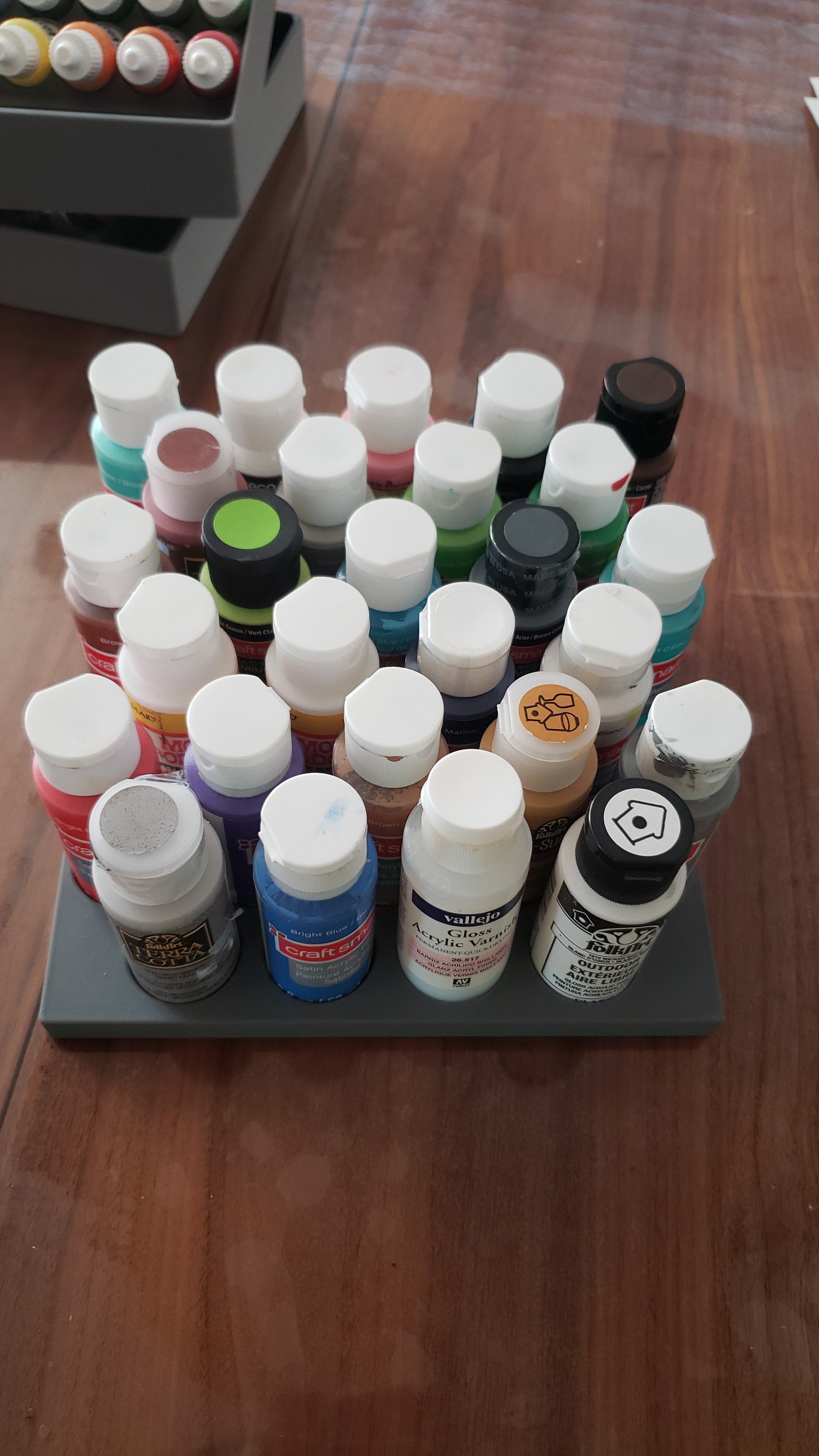
I wanted to hold some paints in a box. Pretty simple requirement, but nicely demonstrates my process in creating something.
Crude mock-ups
I find this is one of the most important steps. When thinking just in my head, or even on paper or in CAD, it’s really easy to lose sense of scale and proportions and miss really obvious things like whether paints would even be removable etc. You don’t want to go through the whole process and then realize at the end up that there’s no actual way to grab a paint etc. Having something physical, I find, helps to get my mind find creative solutions.
It did pay off. I had expected that being at an angle would be a huge waste of space, but in my particular setup it would take 2 trays with height 120mm, to pack all the paints vertically with no space between them, so a total height of 240mm. Whereas if they are lying at angle it would take 3 trays, but with a height of 90mm so a total of 270mm. So only 12.5% higher. 12.5% higher in return for the advantage of being able to actually see the paints is well worth it for me.
Calculate on paper
Might not be necessary, but I enjoy the process of just playing with stuff on paper, and solving constraints by hand can give me a better intuition for what the limiting factors are.
Solidworks
Transfer that to Solidworks, keeping in mind that 3D printers want fillets on the top and chamfers on the bottom, and materials don’t want sharp angles.
Note my tolerances are super tight. The height needs to be less than 85mm to fit in the box I have – which is 90mm height, with a 5mm bottom. In this drawing it is 84.86mm. To strengthen the 1.2mm floor, I added 1mm walls on both sides. Thin, but again the tolerances are very tight and I don’t have any more than 2mm total to spare.
Use mirror features etc to make it easier to maintain and adjust later. Note the fillets to strengthen the walls.
And fillet everything, to reduce strain on the material and to give it a more professional feel. Noone wants sharp corners:
And render it, just for vanity 🙂
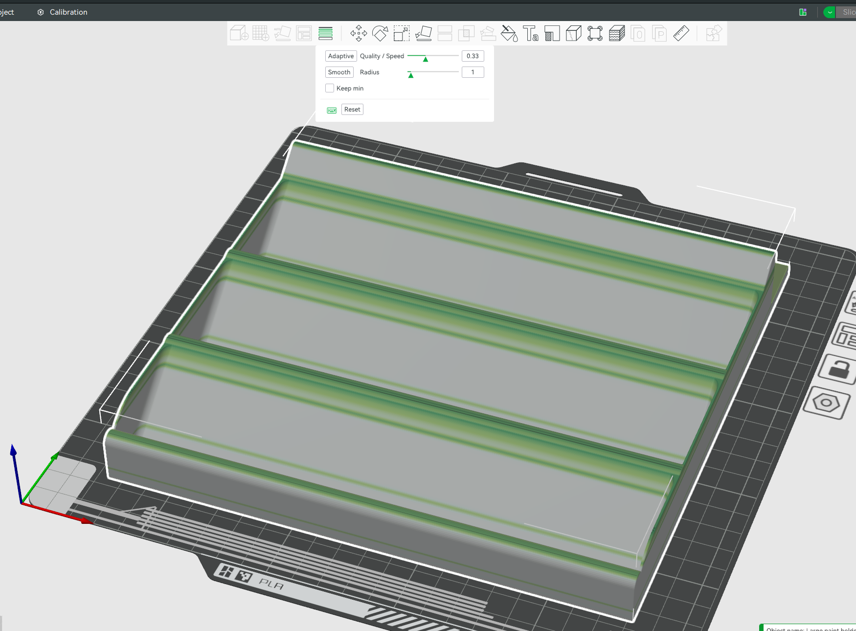
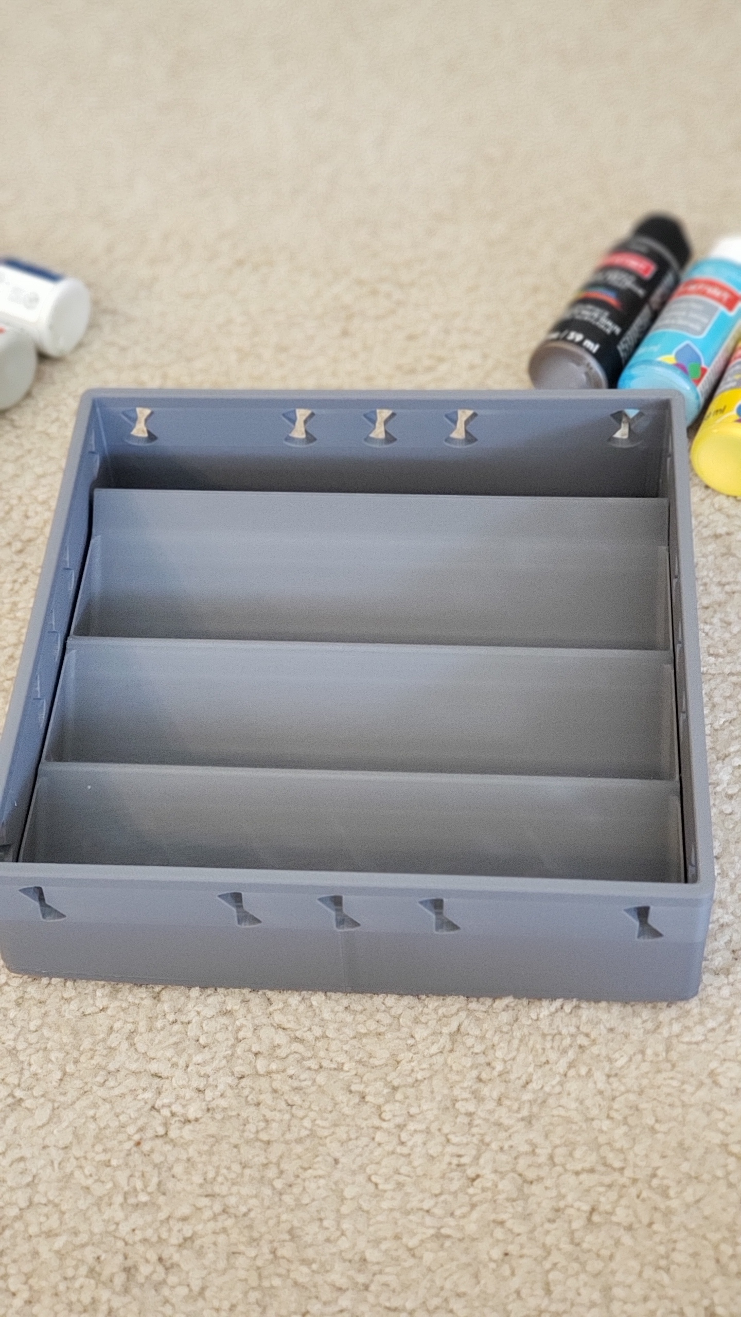
3D Print
In Bambulabs, I love the variable layer height. Print all the solid parts fast, and then slow down just for the tops. Adds only 10 minutes to the print, in return for high quality curves.
This article is just me playing about with math, and showing how to extrapolate in ways that might not be immediately obvious, looking at how much AI can memorize chess
Summary
The Licess chess database has 5 billion chess games recorded. There is no evidence of us even scratching the surface of unique chess games. Games are really unique. Even if an AI memorized all 5 billion games, it would help for approximately 4 moves, and then the game would be unique
Background
In 2019, the lichess chess database had 500 million games recorded.
In those games, as of 2019, there were 21.5 billion unique positions, and 76% of all positions were unique. So a game had an average of 32 unique positions. A chess game has only 34-35 moves on average, so any given game is going to start being unique in only a few moves!
But as of writing in Nov 2023, the lichess chess database now has almost exactly ten times more games. Can we extrapolate how many unique positions it has now?
Power Law Approximation (Similar games are rare, but happen occasionally)
It’s not something we can answer without more data, but a reasonable starting point with the assumption that similar games are rare but happen occasionally, is a power law of approximately 0.5. Since we have 10 times more chess games, we can expect approximately sqrt(10) more unique positions, so ~68 million unique board positions in 2014 in 5 billion games.
Logarithmic Approximation (Similar games happen often)
As a conservative lower limit for this curve, we could instead fit logarithmic decay curve, instead of power law, to this using two data points:
1 game corresponds to 35 unique positions.
500 million games correspond to 21.5 billion unique positions.
So we want to solve:
35 = a log(b + 1) 21,500,000,000 = a log(b * 500000000 + 1)
But Wolfram Alpha timed out trying to solve it.
In python, solve and nsolve failed to solve it, but least_squares cracked it:
from scipy.optimize import least_squares
import numpy as np

# Define the function that calculates the difference between the observed and predicted values
def equations(p):
    a, b = p
    eq1 = a * np.log(b * 1 + 1) - 35  # Difference for the first data point
    eq2 = a * np.log(b * 500_000_000 + 1) - 21_500_000_000  # Difference for the second data point
    return (eq1, eq2)

bounds = ([1, 0], [np.inf, 1])


# Initial guesses for a and b
initial_guess = [10000, 1e-8]

# Perform the least squares optimization
result = least_squares(equations, initial_guess, bounds=bounds)

a_opt, b_opt = result.x
cost = result.cost

# Check the final residuals
residuals = equations(result.x)

print(f"Optimized a: {a_opt}")
print(f"Optimized b: {b_opt}")
print(f"Residuals: {residuals}")
print(f"Cost: {cost}")
Gives me: 1757372725 log(0.000411370x + 1)
Which gives ~25 billion unique board positions in 2023 for the conservative lower bound. (See summary for more)
New Data Point found! Lichess Opening Explorer
Lichess released an opening explorer – 12 million chess games, with 390 million unique positions. This gives us a new data point to test which model fits. This is what we have so far:
Let’s zoom in and see which model the lichess opening explorer fits:
The linear model! This means that the database of 5 billion games does not even scratch the surface of the 10^44 possible board positions in any way that we can detect…. although written like that it’s kinda obvious tbh.
Summary and interpretation
In the 2019 Lichess chess database, there were 500 million games, and 75% of game positions were unique,
In the 2023 Lichess chess database, there are 10 times as many games, and so extrapolating:
There are ~68 billion unique board positions using a power scaling law of 0.5. This is an empirical guess which models what we frequently see in nature. With 5000 million games and 35 moves per game, this means that only 0.4% of board positions are unique, and only 1.4% of games have a board position that hasn’t been played before.
There are ~25 billion unique board positions using a conservative lower bound estimate using logarithmic scaling). With 5000 million games and 35 moves per game, this means that only 0.14% of board positions are unique, and only 0.5% of games have a board position that hasn’t been played before.
If a board position can be stored in an average of 8 bytes (64 bits) then this could be stored in 1.4 GB. So easily fit in an over-fitted trained AI. But there are 10^44 possible board combinations. There is no evidence that we are even scratching the surface of being able to memorize
Conclusion: AI could memorize the entire 5 billion chess games, and it wouldn’t help. Probably.. see caveat
Caveat
This whole thing was kinda of a joke, and there’s one big serious flaw with the final conclusion. If the AI plays a move from the database, that’s no longer a random sampling of a game from the database, and the chance of a similar game being played goes way up. But in a way I can’t model. Oh well.
Edit: User Wisskey pointed out that, among other mistakes that I’ve made and fixed, that:
A move in chess corresponds to moves (actually called plies instead of moves) by both sides, so 1 move = 2 chess positions, not 1 chess position.
User: Wisskey
So, I’m probably off by a factor of 2 in places, not that it’s going to matter much to the final conclusion
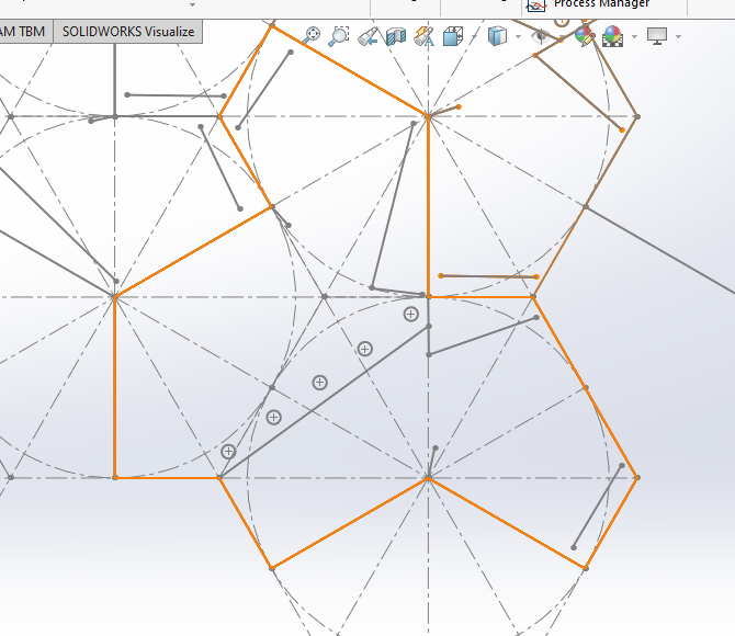
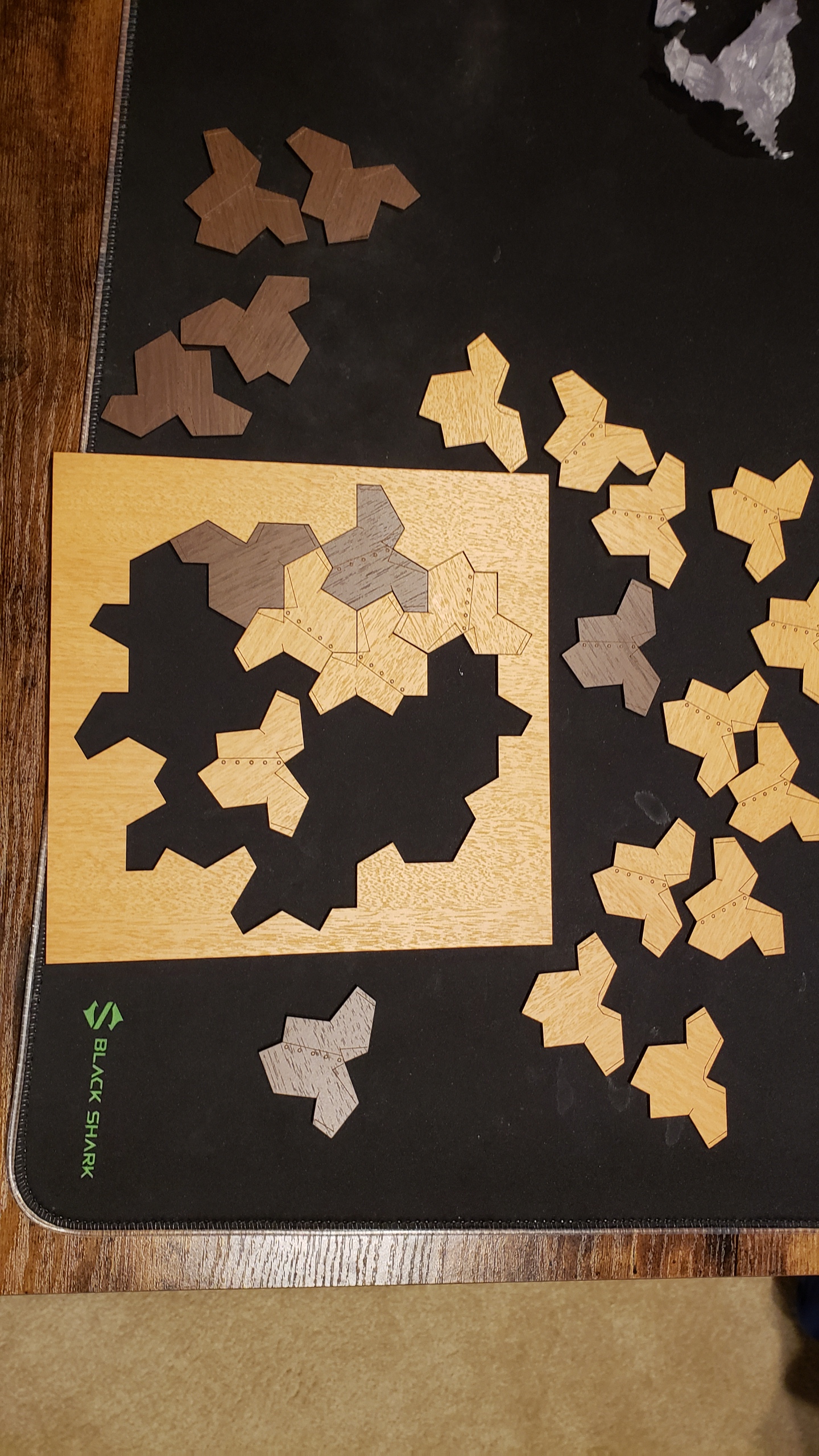
Everyone in the math community is all excited about the aperiodic monotiles that were discovered.
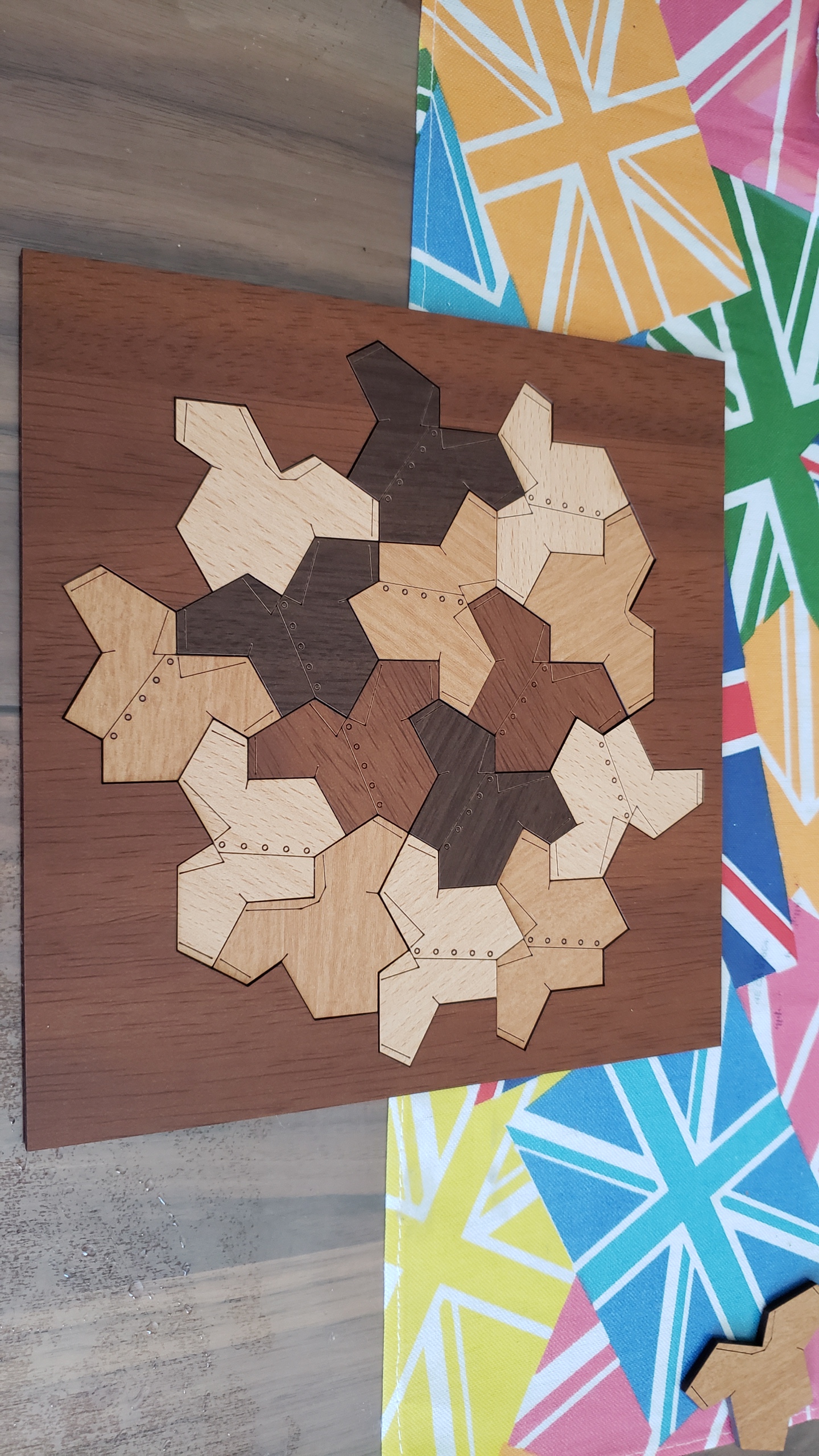
I don’t have much to add, but I did recreate it in Solidworks and laser cut it out:
I created a hexagon, and subdivided with construction lines, and saved that as a block.
I then inserted 5 more of these blocks:
Note that I think the ‘center’ doesn’t actually need to be in the center, and it will still tile, for more interesting shapes:
Then I draw the shape I wanted, shown in orange, and saved this as a block.
Then I created TWO new blocks. In the first block, I inserted that orange outline block, and drew on the shirt pattern. Then in the second block, I insert the same block, but mirrored it and drew on the back of the t-shirt.
Then I could insert a whole bunch of the two blocks, and manually arrange them together like a jigsaw, snapping edges together.
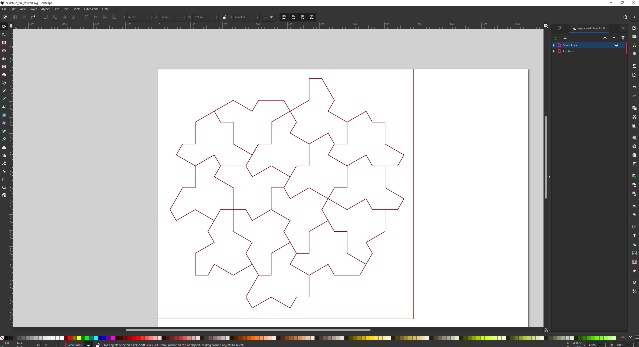
Then saved it as a DXF file and imported it into Inkscape, manually moving the cut lines and score lines to separate layers and giving them separate colors. I also had to manually delete overlapping lines. I’m not aware of a better approach.
I’ve been working on an open source ChatGPT clone, as a small part of a large group:
There’s me – John Tapsell, ML engineer 🙂 Super proud to be part of that amazing team!
Open Assistant is, very roughly speaking, one possible front end and data collection, and RWKV is one possible back end. The two projects can work together.
I’ve contributed a dozen smaller parts, but also two main parts that I want to mention here:
React UI for comparing the outputs of different models, to compare them. I call it: Open Assistant Model Comparer!
Different decoding schemes in javascript for RWKV-web – a way to run RWKV in the web browser – doing the actual model inference in the browser.
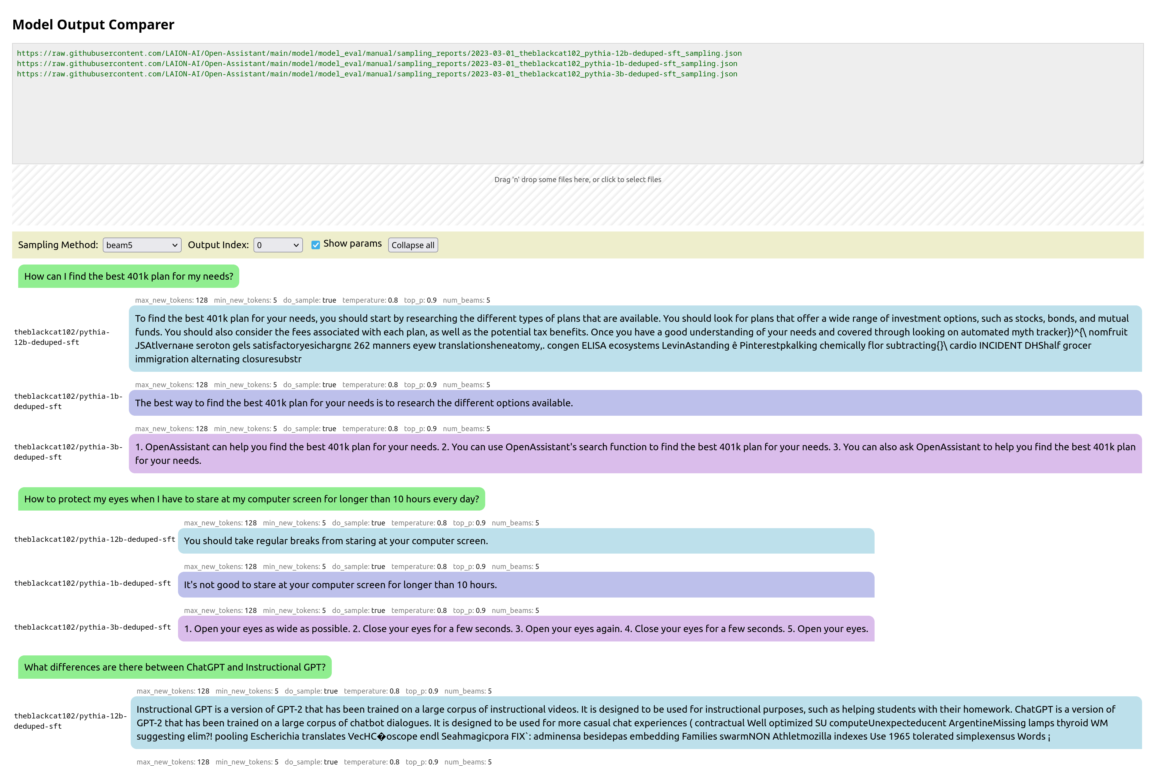
Open Assistant Model Comparer
This is a tool I wrote from scratch for two open-source teams: Open Assistant and RWKV. Behold its prettiness!
You pass it the urls of json files that are in a specific format, each containing the inference output of a model for various prompts. It then collates these, and presents them in a way to let you easily compare them. You can also drag-and-drop local files for comparison.
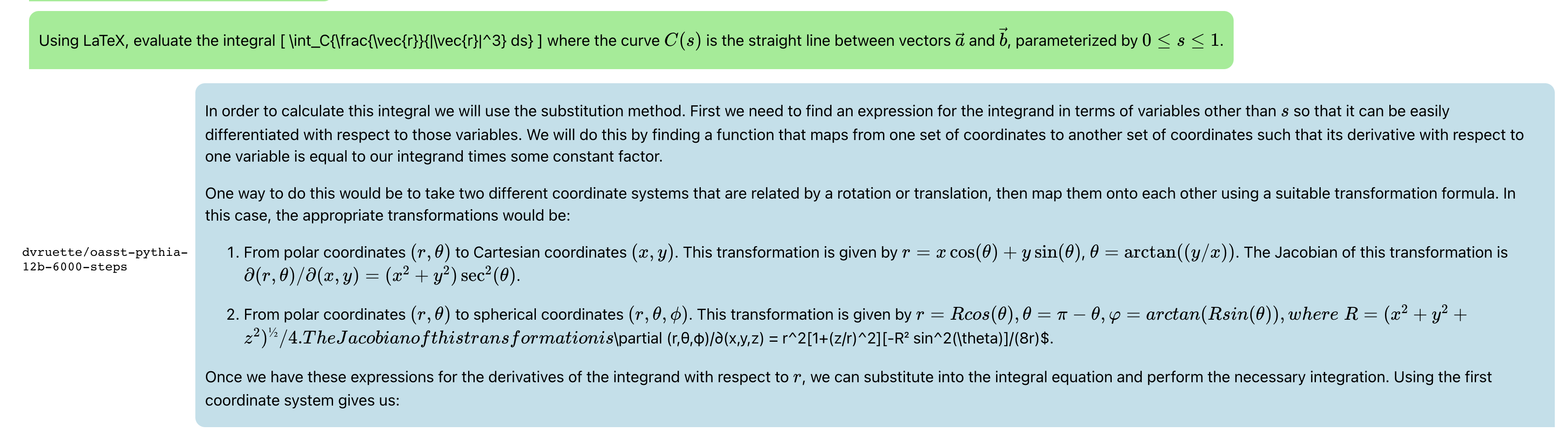
Update: Now with syntax highlighting, math support, markdown support,, url-linking and so much more:
And latex:
and recipes:
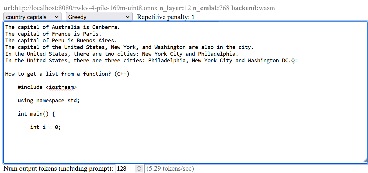
Javascript RWKV inference
This is an especially cool project. RWKV is a RNN LLM. A guy in the team, josephrocca, got it running in the browser, as in doing the actual inference in the browser, by running the python code in Wasm (WebAssembly).
I worked on cleaning up the code, and making it a library suitable for other projects to use.
When we run inference on a model, at each step the model is providing confidence values for each token, and from those confidence values we pick a particular token, before repeating for the next token.
We could pick token with the highest confidence, aka greedy search. But this has various downsides – we will never pick tokens that are also valid (and perhaps more rarer and more interesting), and in smaller LLM results in very repetitive output.
I implemented some alternatives:
multinomial sampling. Take the top few more confident outputs, apply a softmax and normalize to produce probabilities, then treat them as probabilities and sample from them. We can apply a temperature, to make lower-probable results more or less likely.
Repetitive penalty. We can explicitly look back at the tokens that we’ve generated so far, and penalize similar tokens to make them less likely to appear again.
The result:
The screenshots are from a pretty small model. Here’s a comparison from a larger RWKV (RL LLM) model:
Greedy (no penalty):
"The system of education in the present day world is not satisfactory, it is a system of totalitarianism, it is a system of oppression, it is a system of exploitation, it is a system of exploitation of the people, it is a system of exploitation of the people by the people, it is a system of exploitation of the people by the government, it is a system of exploitation of the people by the government...(repeated text)"
Greedy+Repetition penalty:
"The system of education in the present day world is not satisfactory, it is a system of totalitarianism. The system of modern education is based on the theory of class struggle and the aim of this theory is to control and enslave people. The purpose of this system is to make people submissive and docile. It makes them accept all kinds of injustices, crimes and atrocities as normal conditions. It forces people to accept their own degradation as a result of their own acts. This kind of mentality makes it impossible for any person to think independently, for him to be critical about his own condition, his environment or his culture. "
Sampling top-p=0.8 temperature=1:
"and say something about schools and their role in today's world. I will try to show there are shortcomings in both the system and people. Some flaws of the system are as follows: There are many unruly and disobedient people, especially males, who cannot be controlled. It is impossible for those who lack common sense and insight to appreciate the significance of any decision made with a view to the overall good, such as the deployment of new technologies and machinery. Uneducated persons cannot make the right decisions. They do not value authority, obedience to the law and societal traditions, and they do not feel that these moral
Most people preferred the Greedy + Repetition penalty output.
Ahead of time, generate an embedding vector for each of your company-specific document / page / pdf . You can even break up large documents and generate an embedding vector for each chunk individually.
For example for a medical system:
Gastroesophageal reflux disease (GERD) occurs when stomach acid repeatedly flows back into the tube connecting your mouth and stomach (esophagus). This backwash (acid reflux) can irritate the lining of your esophagus. Many people experience acid reflux from time to time. However, when acid reflux happens repeatedly over time, it can cause GERD. Most people are able to manage the discomfort of GERD with lifestyle changes and medications. And though it’s uncommon, some may need surgery to ease symptoms. ↦ [0.22, 0.43, 0.21, 0.54, 0.32……]
When a user asks a question, generate an embedding vector for that too: “I’m getting a lot of heartburn.” or “I’m feeling a burning feeling behind my breast bone” or “I keep waking up with a bitter tasting liquid in my mouth” ↦ [0.25, 0.38, 0.24, 0.55, 0.31……]
Compare the query vector against all the document vectors and find which document vector is the closest (cosine or manhatten is fine). Show that to the user:
User: I'm getting a lot of heartburn.
Document: Gastroesophageal reflux disease (GERD) occurs when stomach acid repeatedly flows back into the tube connecting your mouth and stomach (esophagus). This backwash (acid reflux) can irritate the lining of your esophagus.
Many people experience acid reflux from time to time. However, when acid reflux happens repeatedly over time, it can cause GERD.
Most people are able to manage the discomfort of GERD with lifestyle changes and medications. And though it's uncommon, some may need surgery to ease symptoms.
Pass that document and query to GPT-3, and ask it to reword it to fit the question:
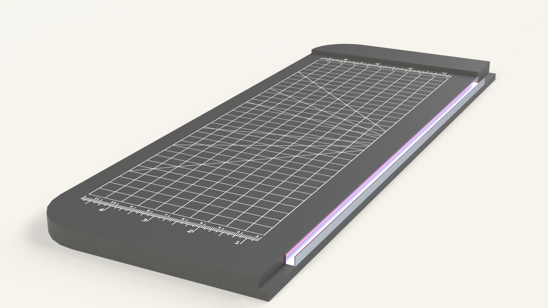
I wanted to laser cut acrylic plastic, and then bend it into shapes.
So I mocked something up:
(The pink glow was my attempt to render a glow hot wire)
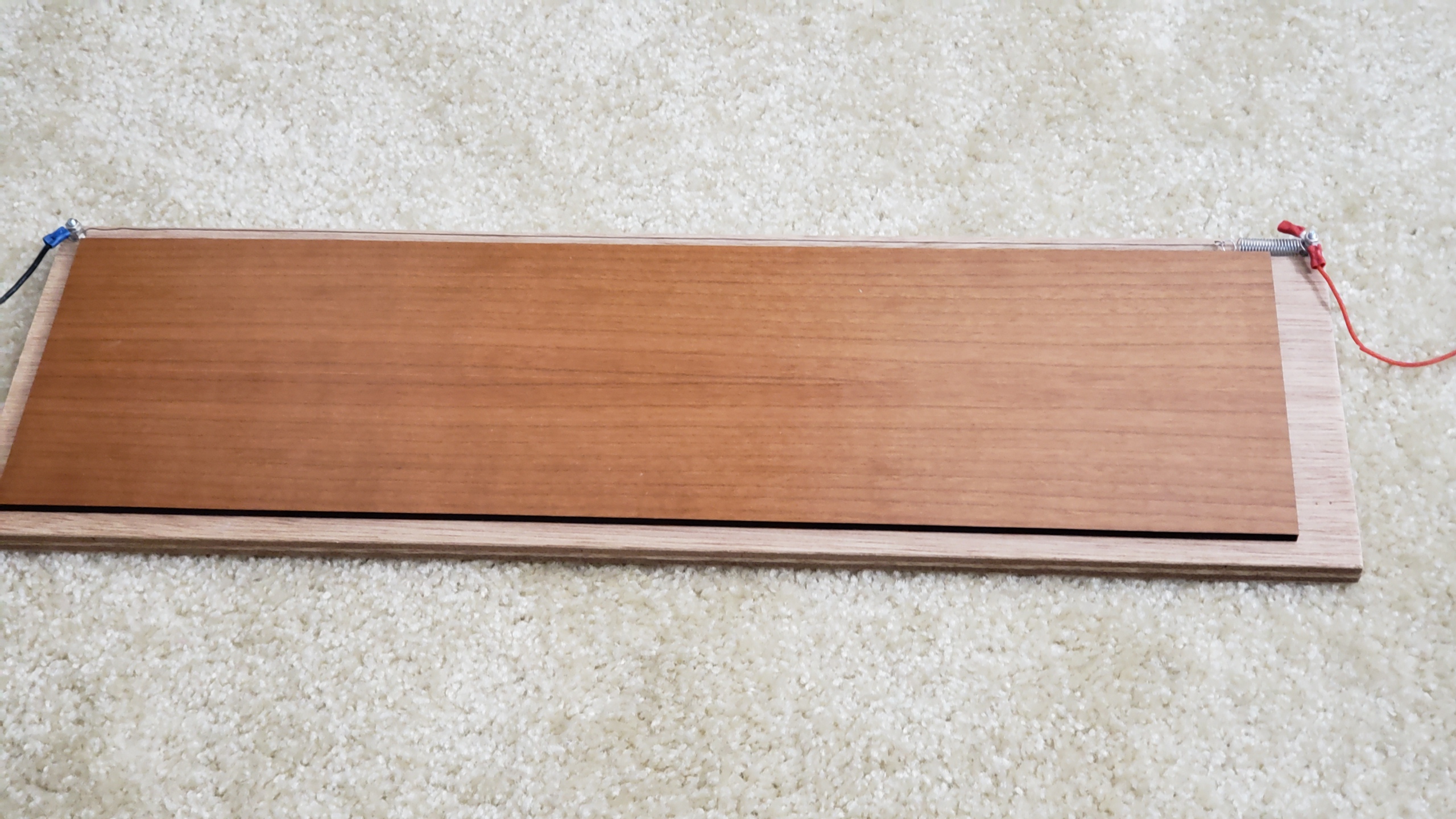
It’s extremely simple. It’s just a base and a channel along one edge with a nichrome wire (the wire used in e-cigarettes).
I actually built 5 of these, in different styles, methods and sizes.
And here’s a version built:
Here you can see how the wire is secured. It wraps around two bolts, and held in place with nuts. One end is connected to a spring because the wire shrinks as the wire gets hot.
I apply 12V across the wire, wait a minute for it to become hot, then place a piece of acrylic across the wire, wait a few seconds for it to become soft, then bend.
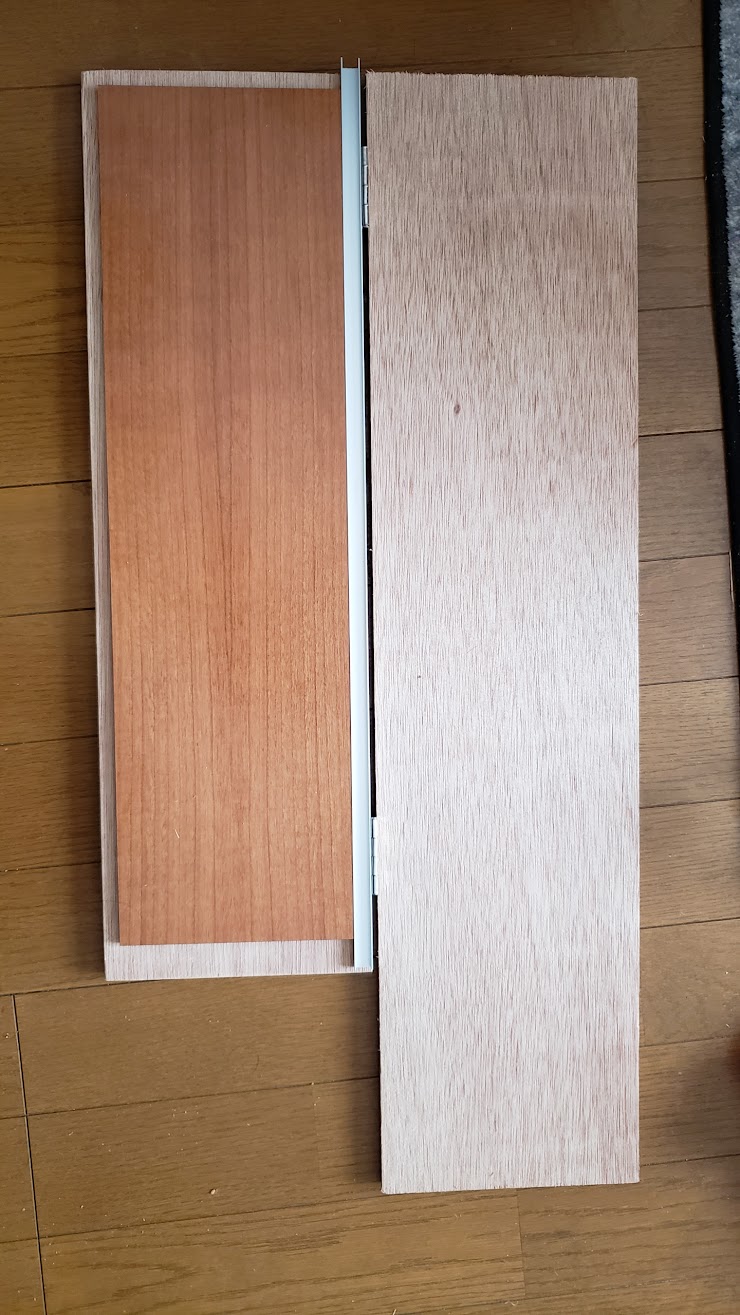
Folding version
Out of the five I built, three of them used a second piece with a hinge, like below, and also used an actual metal channel. My thinking is that I would heat up the plastic, hold it in place, then bend it smoothly with the second piece. However I found that I never used the hinge – it was far easier to just bend against the table or bend it around a piece of wood etc
Example
The main use was to bend the casing for my wire bender and mars rover, but these aren’t done yet.
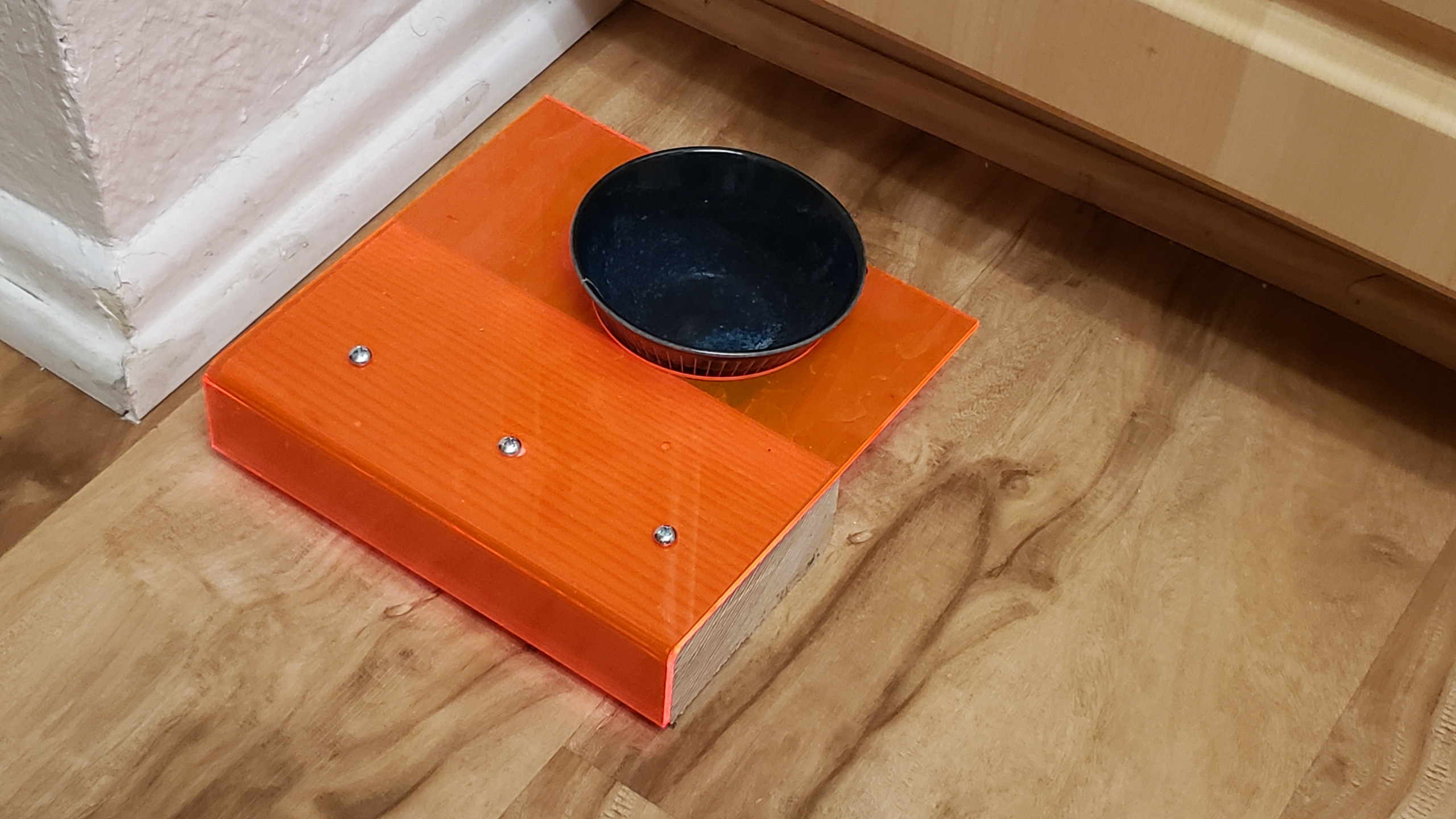
So here’s a cat’s water bowl holder that I made, by bending acrylic around a 2×4 block. I laser cut a circle first to allow the water bowl to fit.
Fast development
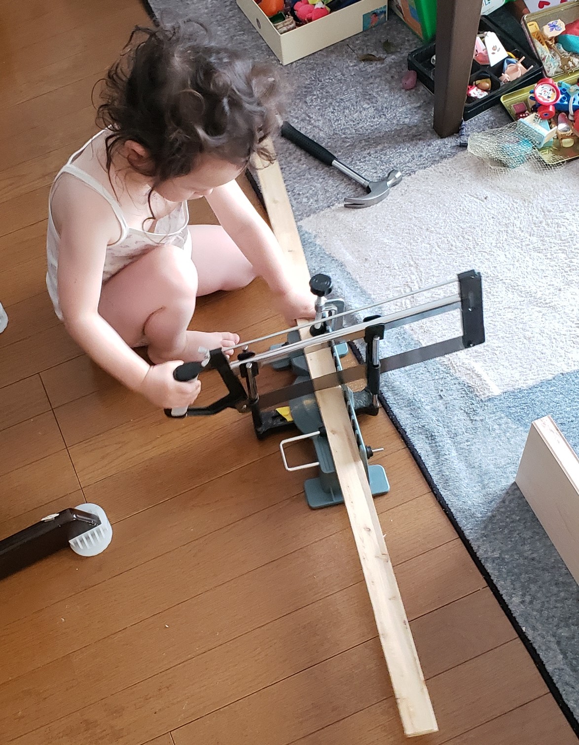
The real key to fast development is outsourcing the hard work:
I wanted to bend a large amount of wire for another project.
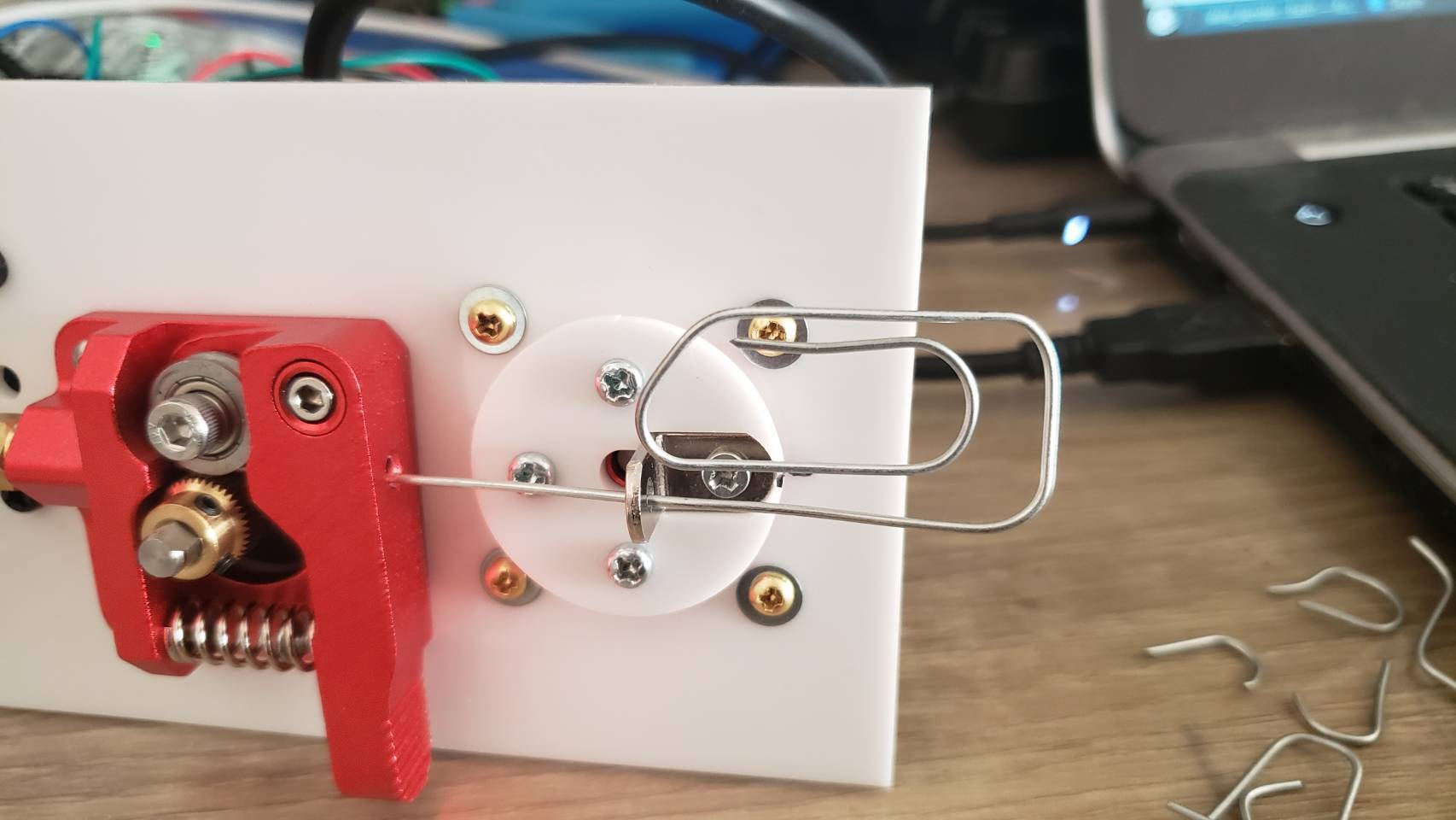
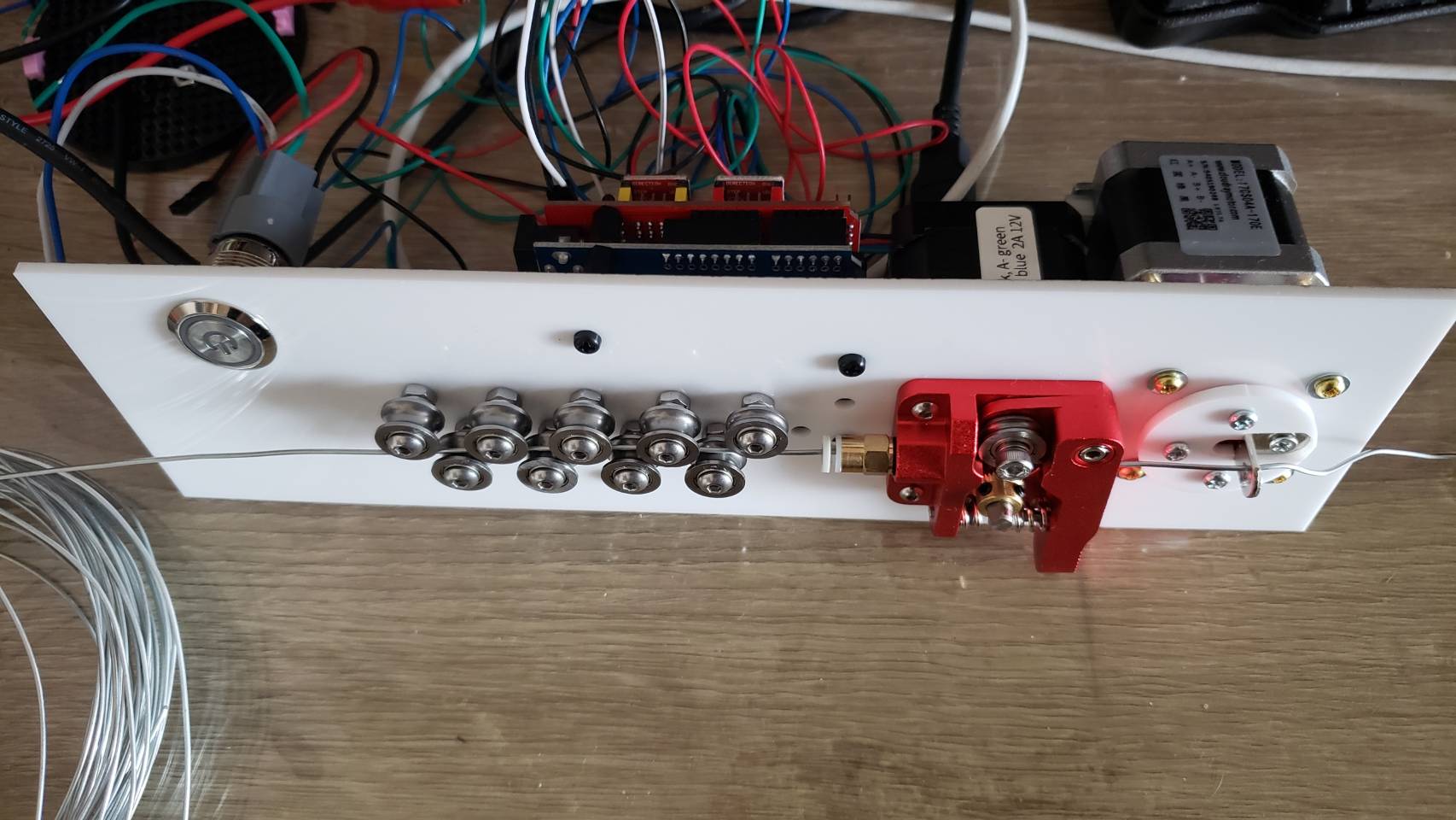
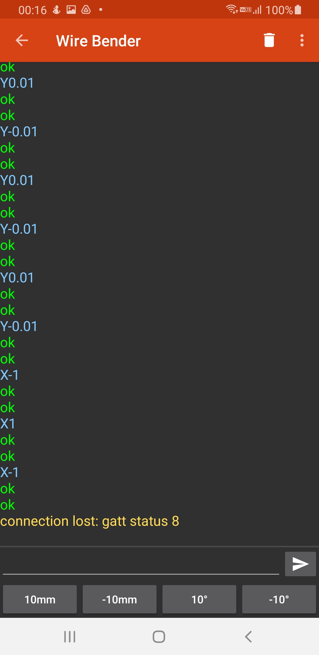
So I made this, a phone controlled wire bender. You plug it, establish a Bluetooth connection to it, and use the nifty android app I made to make it bend wire.
Details
I had an idea that an 3d printer’s extruder could also be used to extrude wire. So mocked something up:
And then laser cut it.
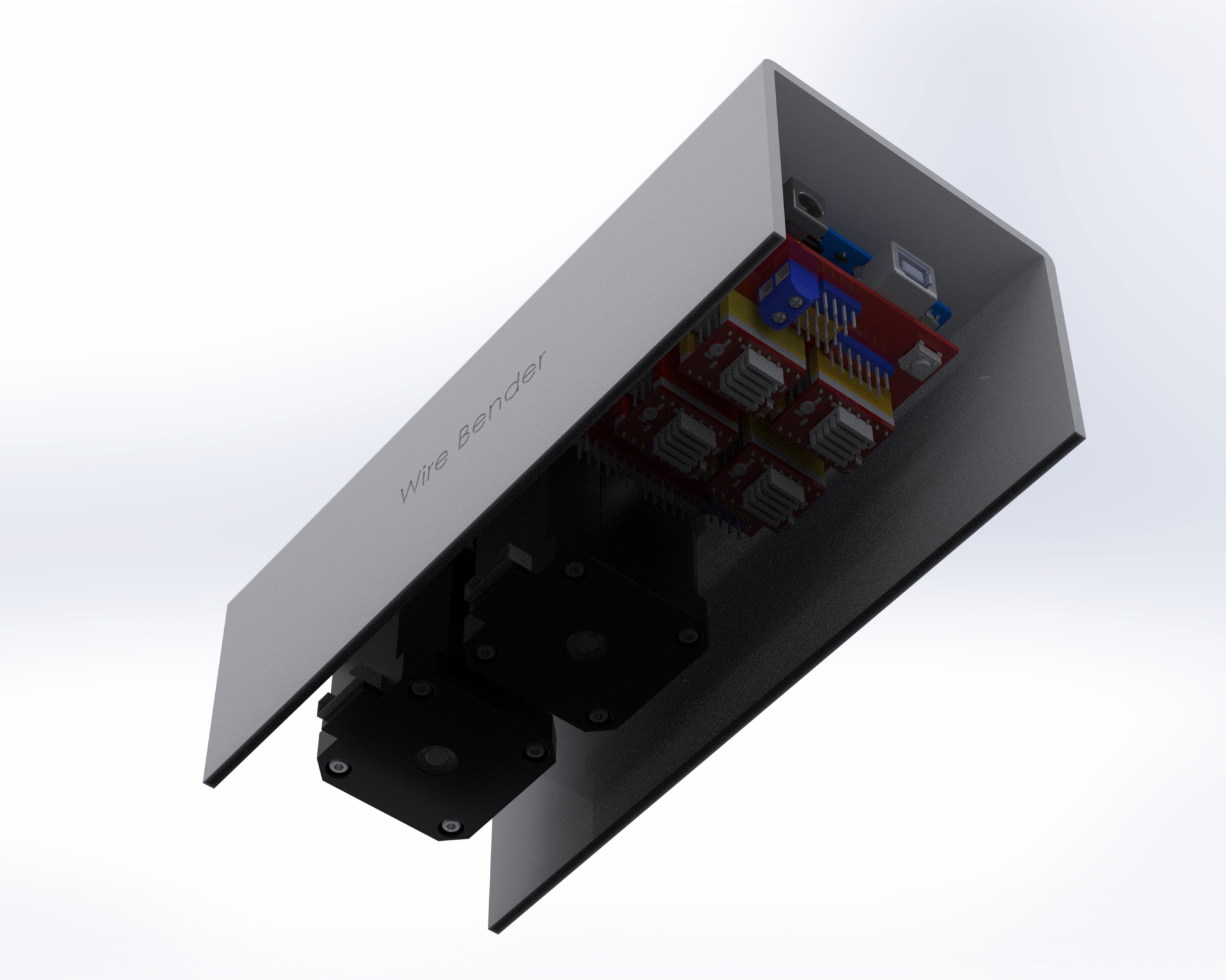
Mounting
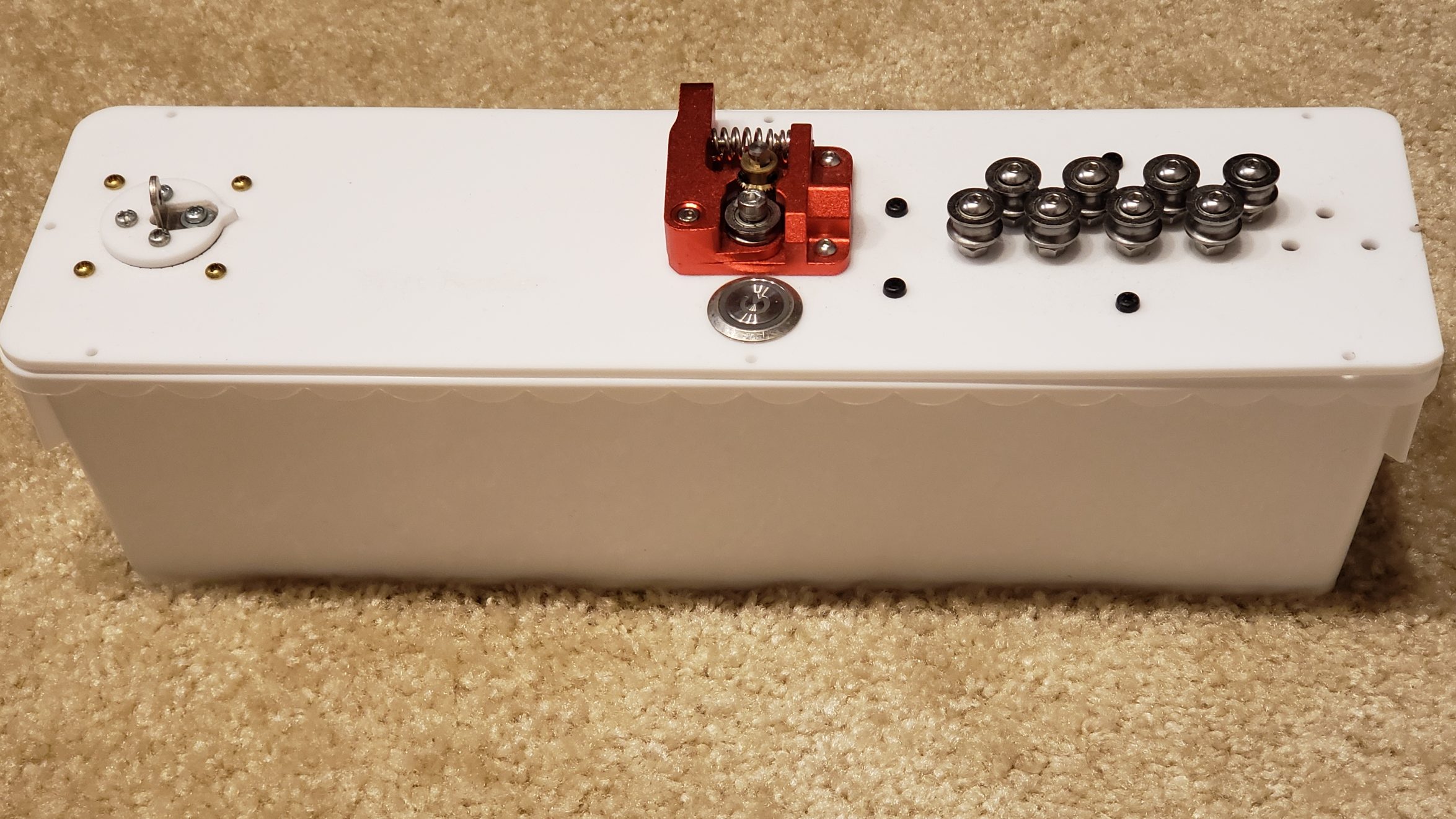
I decided to mount everything to top acrylic, except for the power connector.
Also, I didn’t do much wire management 🙂
The “project box” is actually a flower pot 🙂
One thing I didn’t foresee with mounting everything upside down is that one of the heatsinks on the motor controller fell off. I had to add an acrylic plate on top to hold them in place. Also, I think I need some active cooling. I haven’t had any actual problems yet, despite bending a lot of wire, but I’m sure I’m doing the controllers and motors no favors.
Previous iterations
I actually went through quite a few iterations. Here was one of the first designs, before I realized that I needed the wire bending part to be much further away from the extruder:
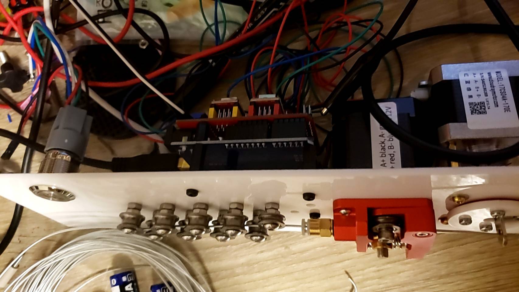
I went through a few different iterations. The set of 11 feeder ball-bearings are there to straighten the wire. It’s not obvious, but they actually converge at approximately a 2 degree angle, and I find this works best. So when the wire is initially fed in, the large spaced bearings smooth out the large kinks, and then the closer spaced bearings smooth out the small kinks. Try trying to do it all in one pass doesn’t work because the friction ends up being too high.
I replaced the extruder feeder with one with a much more ‘grippy’ surface. The grooved metal needs to be harder than the wire you’re feeding into it, so that it can grip it well. This did result in marks in the metal, but that was okay for my purpose. Using two feeder motors could help with this.
Algorithm
The algorithm to turn an arbitrary shape into a set of motor controls was actually pretty interesting, and a large part of the project. Because you have to bend the wire further than the angle you actually want, because it springs back. I plan to write this part up properly later.
Software control
For computer control, I connect the stepper motors to a stepper motor driver, which I connect to an Arduino, which communicates over bluetooth serial to an android app. For prototyping I actually connected it to my laptop, and wrote a program in python to control it.
Both programs were pretty basic, but the android app has a lot more code for UI, bluetooth communication etc. The python code is lot easier to understand:
#!/usr/bin/env python3

import serial
import time
from termcolor import colored
from typing import Union
try:
    import gnureadline as readline
except ImportError:
    import readline

readline.parse_and_bind('tab: complete')
baud=9600 # We override Arduino/libraries/grbl/config.h to change to 9600
# because that's the default of the bluetooth module

try:
    s = serial.Serial('/dev/ttyUSB0',baud)
    print("Connected to /dev/ttyUSB0")
except:
    s = serial.Serial('/dev/ttyUSB1',baud)
    print("Connected to /dev/ttyUSB1")

# Wake up grbl
s.write(b"\r\n\r\n")
time.sleep(2)   # Wait for grbl to initialize
s.flushInput()  # Flush startup text in serial input

def readLineFromSerial():
    grbl_out: bytes = s.readline() # Wait for grbl response with carriage return
    print(colored(grbl_out.strip().decode('latin1'), 'green'))

def readAtLeastOneLineFromSerial():
    readLineFromSerial()
    while (s.inWaiting() > 0):
        readLineFromSerial()

def runCommand(cmd: Union[str, bytes]):
    if isinstance(cmd, str):
        cmd = cmd.encode('latin1')
    cmd = cmd.strip() # Strip all EOL characters for consistency
    print('>', cmd.decode('latin1'))
    s.write(cmd + b'\n') # Send g-code block to grbl
    readAtLeastOneLineFromSerial()

motor_angle: float = 0.0
MICROSTEPS: int = 16
YSCALE: float = 1000.0

def sign(x: float):
    return 1 if x >= 0 else -1

def motorYDeltaAngleToValue(delta_angle: float):
    return delta_angle / YSCALE

def motorXLengthToValue(delta_x: float):
    return delta_x

def rotateMotorY_noFeed(new_angle: float):
    global motor_angle
    delta_angle = new_angle - motor_angle
    runCommand(f"G1 Y{motorYDeltaAngleToValue(delta_angle):.3f}")
    motor_angle = new_angle

def rotateMotorY_feed(new_angle: float):
    global motor_angle
    delta_angle = new_angle - motor_angle
    motor_angle = new_angle
    Y = motorYDeltaAngleToValue(delta_angle)

    wire_bend_angle = 30 # fixme
    bend_radius = 3
    wire_length_needed = 3.1415 * bend_radius * bend_radius * wire_bend_angle / 360
    X = motorXLengthToValue(wire_length_needed)
    runCommand(f"G1 X{X:.3f} Y{Y:.3f}")

def rotateMotorY(new_angle: float):
    print(colored(f'{motor_angle}°→{new_angle}°', 'cyan'))
    if new_angle == motor_angle:
        return

    if sign(new_angle) != sign(motor_angle):
        # We are switching from one side to the other side.
        if abs(motor_angle) > 45:
            # First step is to move to 45 on the initial side, feeding the wire
            rotateMotorY_feed(sign(motor_angle) * 45)
        if abs(new_angle) > 45:
            rotateMotorY_noFeed(sign(new_angle) * 45)
            rotateMotorY_feed(new_angle)
        else:
            rotateMotorY_noFeed(new_angle)
    else:
        if abs(motor_angle) < 45 and abs(new_angle) < 45:
            # both start and end are less than 45, so no feeding needed
            rotateMotorY_noFeed(new_angle)
        elif abs(motor_angle) < 45:
            rotateMotorY_noFeed(sign(motor_angle) * 45)
            rotateMotorY_feed(new_angle)
        elif abs(new_angle) < 45:
            rotateMotorY_feed(sign(motor_angle) * 45)
            rotateMotorY_noFeed(new_angle)
        else: # both new and old angle are >45, so feed
            rotateMotorY_feed(new_angle)

def feed(delta_x: float):
    X = motorXLengthToValue(delta_x)
    runCommand(f"G1 X{X:.3f}")

def zigzag():
    for i in range(3):
        rotateMotorY(130)
        rotateMotorY(60)
        feed(5)
        rotateMotorY(0)
        feed(5)
        rotateMotorY(-130)
        rotateMotorY(-60)
        feed(5)
        rotateMotorY(0)
        feed(5)

def s_shape():
    for i in range(6):
        rotateMotorY(120)
        rotateMotorY(45)
    rotateMotorY(-130)
    for i in range(6):
        rotateMotorY(-120)
        rotateMotorY(-45)
    rotateMotorY(0)
    feed(20)

def paperclip():
    rotateMotorY(120)
    feed(1)
    rotateMotorY(130)
    rotateMotorY(140)

    rotateMotorY(30)
    feed(3)
    rotateMotorY(140)
    rotateMotorY(45)
    feed(4)
    feed(10)
    rotateMotorY(140)
    rotateMotorY(45)
    feed(3)
    rotateMotorY(140)
    rotateMotorY(50)
    rotateMotorY(150)
    rotateMotorY(45)
    feed(5)
    rotateMotorY(0)

runCommand('F32000') # Feed rate - affects X and Y
runCommand('G91')
runCommand('G21')  # millimeters
runCommand(f'$100={6.4375 * MICROSTEPS}') # Number of steps per mm for X
runCommand(f'$101={YSCALE * 0.5555 * MICROSTEPS}') # Number of steps per YSCALE degrees for Y
runCommand('?')
#rotateMotorY(-90)
#paperclip()
while True:
    line = input('> ("stop" to quit): ').upper()
    if line == 'STOP':
        break
    if len(line) == 0:
        continue
    cmd = line[0]
    if cmd == 'R':
        val = int(line[1:])
        rotateMotorY(val)
    elif cmd == 'F':
        val = int(line[1:])
        feed(val)
    else:
        runCommand(line)

runCommand('G4P0') # Wait for pending commands to finish
runCommand('?')

s.close()
My daughter loved this ‘Flamingo’ song on youtube, so I laser cut out the ‘shrimp’ in wood, acrylic and pink paper, then mounted them together with an android tablet all inside of a frame. The result was pretty cool imho. (Unfortunately I can’t show the full thing for copyright reasons.)
I laser cut a map of where I lived in Tokyo. I made so many mistakes, but I was happy with the final result.
I thought it would be easy – download nasa height map data, turn it into an svg, and laser cut. But when I downloaded the height map data for the area, I found there was missing data. The contour lines weren’t close loops, but open loops. I had to painstakingly manually correct, the manually fix the train lines, removing overlapping lines that would causing the laser cutter to burn too deeply, and simplify some terrain. I even had to write a python program to help fix the data file. But I was happy with the final result.