I’ve been working on an open source ChatGPT clone, as a small part of a large group:

Open Assistant is, very roughly speaking, one possible front end and data collection, and RWKV is one possible back end. The two projects can work together.
I’ve contributed a dozen smaller parts, but also two main parts that I want to mention here:
- React UI for comparing the outputs of different models, to compare them. I call it: Open Assistant Model Comparer!
- Different decoding schemes in javascript for RWKV-web – a way to run RWKV in the web browser – doing the actual model inference in the browser.
Open Assistant Model Comparer
This is a tool I wrote from scratch for two open-source teams: Open Assistant and RWKV. Behold its prettiness!
It’s hosted here: https://open-assistant.github.io/oasst-model-eval/ and github code here: https://github.com/Open-Assistant/oasst-model-eval
You pass it the urls of json files that are in a specific format, each containing the inference output of a model for various prompts. It then collates these, and presents them in a way to let you easily compare them. You can also drag-and-drop local files for comparison.
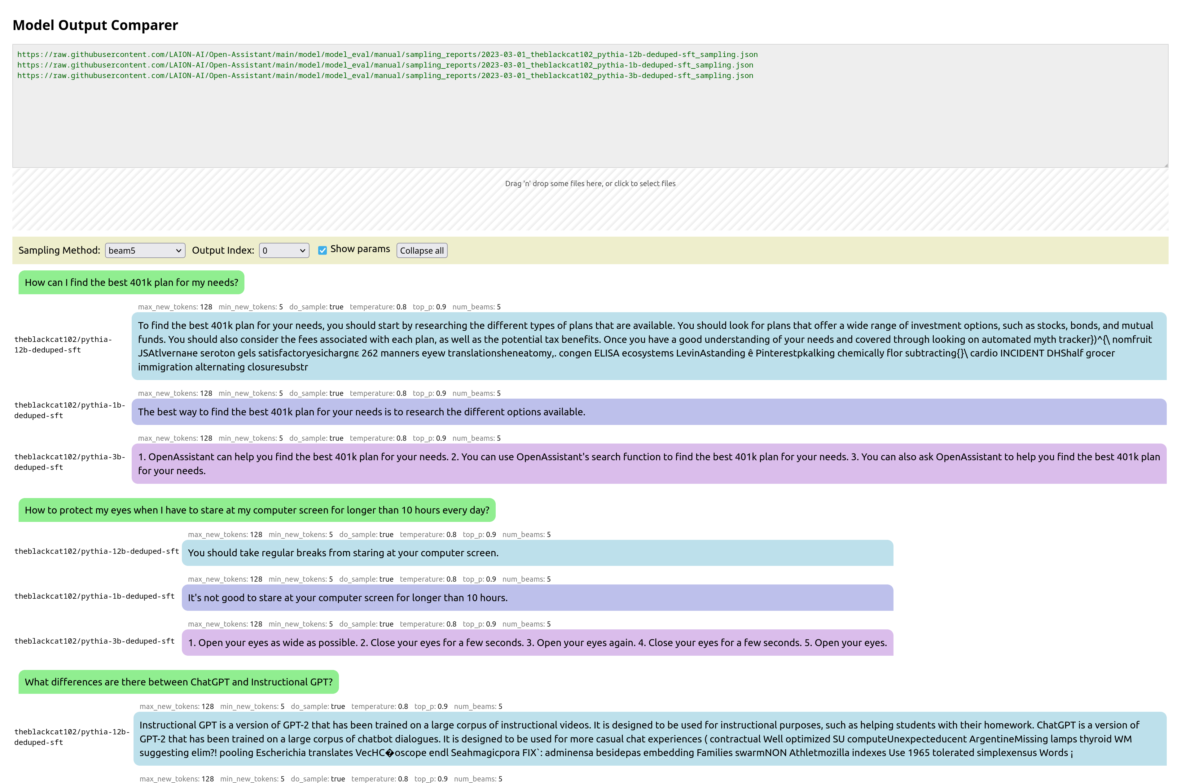
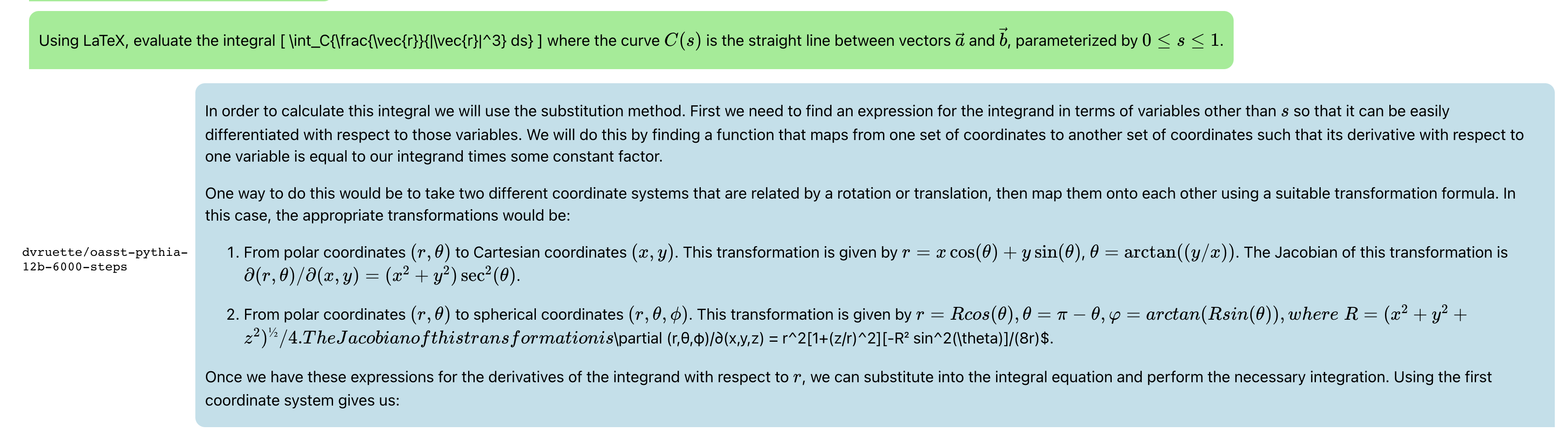
Update: Now with syntax highlighting, math support, markdown support,, url-linking and so much more:

And latex:
and recipes:

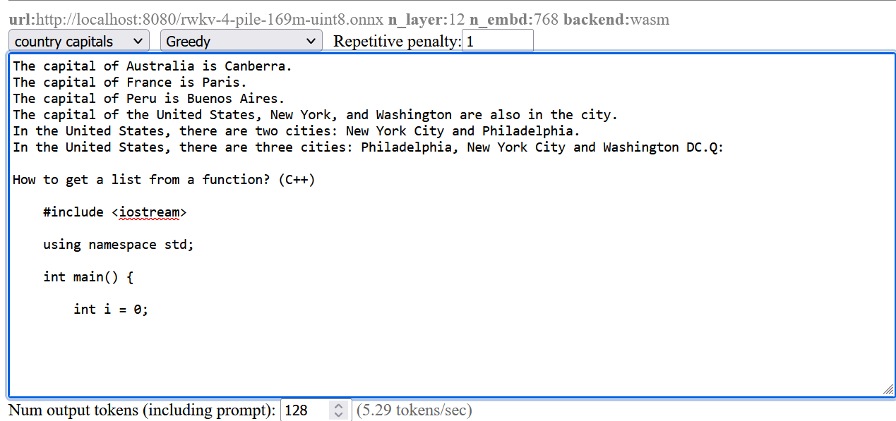
Javascript RWKV inference
This is an especially cool project. RWKV is a RNN LLM. A guy in the team, josephrocca, got it running in the browser, as in doing the actual inference in the browser, by running the python code in Wasm (WebAssembly).
I worked on cleaning up the code, and making it a library suitable for other projects to use.
Project is here: https://github.com/josephrocca/rwkv-v4-web
Then I looked inference decoding:
When we run inference on a model, at each step the model is providing confidence values for each token, and from those confidence values we pick a particular token, before repeating for the next token.
We could pick token with the highest confidence, aka greedy search. But this has various downsides – we will never pick tokens that are also valid (and perhaps more rarer and more interesting), and in smaller LLM results in very repetitive output.
I implemented some alternatives:
- multinomial sampling. Take the top few more confident outputs, apply a softmax and normalize to produce probabilities, then treat them as probabilities and sample from them. We can apply a temperature, to make lower-probable results more or less likely.
- Repetitive penalty. We can explicitly look back at the tokens that we’ve generated so far, and penalize similar tokens to make them less likely to appear again.
The result:

The screenshots are from a pretty small model. Here’s a comparison from a larger RWKV (RL LLM) model:
Greedy (no penalty):
"The system of education in the present day world is not satisfactory, it is a system of totalitarianism, it is a system of oppression, it is a system of exploitation, it is a system of exploitation of the people, it is a system of exploitation of the people by the people, it is a system of exploitation of the people by the government, it is a system of exploitation of the people by the government...(repeated text)"
Greedy+Repetition penalty:
"The system of education in the present day world is not satisfactory, it is a system of totalitarianism. The system of modern education is based on the theory of class struggle and the aim of this theory is to control and enslave people. The purpose of this system is to make people submissive and docile. It makes them accept all kinds of injustices, crimes and atrocities as normal conditions. It forces people to accept their own degradation as a result of their own acts. This kind of mentality makes it impossible for any person to think independently, for him to be critical about his own condition, his environment or his culture. "
Sampling top-p=0.8 temperature=1:
"and say something about schools and their role in today's world. I will try to show there are shortcomings in both the system and people. Some flaws of the system are as follows: There are many unruly and disobedient people, especially males, who cannot be controlled. It is impossible for those who lack common sense and insight to appreciate the significance of any decision made with a view to the overall good, such as the deployment of new technologies and machinery. Uneducated persons cannot make the right decisions. They do not value authority, obedience to the law and societal traditions, and they do not feel that these moral
Most people preferred the Greedy + Repetition penalty output.


 if the image is that of a cat.
 , in the network so that it slightly decreases the error (
 ). And then repeat.

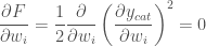
 (or if it equals 0, we need to consider the third differential etc).
 , we’ll use
  to be the half squared error of
  .
.


 and
and  are learning rate hyperparameters.
 i.e. That it tends to 1 as x approaches positive infinity
 i.e. That it tends to 0 as x approaches negative infinity
 and
and 
 .
.
 and
and 


 then
then  . I was too lazy to update the graphs sorry)
 :
:
 ).
).
![[1,1]/\sqrt{2}](https://s0.wp.com/latex.php?latex=%5B1%2C1%5D%2F%5Csqrt%7B2%7D&bg=ffffff&fg=444444&s=0&c=20201002) and
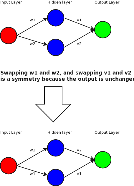
and ![[1,-1]/\sqrt{2}](https://s0.wp.com/latex.php?latex=%5B1%2C-1%5D%2F%5Csqrt%7B2%7D&bg=ffffff&fg=444444&s=0&c=20201002) . Or in pictures:
. Or in pictures:
