This is a random idea that I’ve been thinking about. A reader messaged me to say that this look similar to online l-bgfs. To my inexperienced eyes, I can’t see this myself, but I’m still somewhat a beginner.

Yes, I chose a cat example simply so that I had an excuse to add cats to my blog.

Say we are training a neural network to take images of animals and classify the image as being an image of a cat or not a cat.

You would train the network to output, say, if the image is that of a cat.

To do so, we can gather some training data (images labelled by humans), and for each image we see what our network predicts (e.g. “I’m 40% sure it’s a cat”).  We compare that against what a human says (“I’m 100% sure it’s a cat”)  find the squared error (“We’re off by 0.6, so our squared error is 0.6^2”) and adjust each parameter, , in the network so that it slightly decreases the error ().  And then repeat.

It’s this adjustment of each parameter that I want to rethink.  The above procedure is Stochastic Gradient Descent (SGD) – we adjust to reduce the error for our test set (I’m glossing over overfitting, minibatches, etc).

My idea is to encode this into the SGD update. To find a local minima for a particular test image we want:

(or if it equals 0, we need to consider the third differential etc).

Let’s concentrate on just the first criteria for the moment. Since we’ve already used the letter to mean the half squared error of , we’ll use to be the half squared error of .

So we want to minimize the half squared error :

So to minimize we need the gradient of this error:

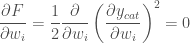
Applying the chain rule:

Conclusion

We finished with a new SGD update rule. I have no idea if this actually will be any better, and the only way to find out is to actually test. This is left as an exercise for the reader 😀