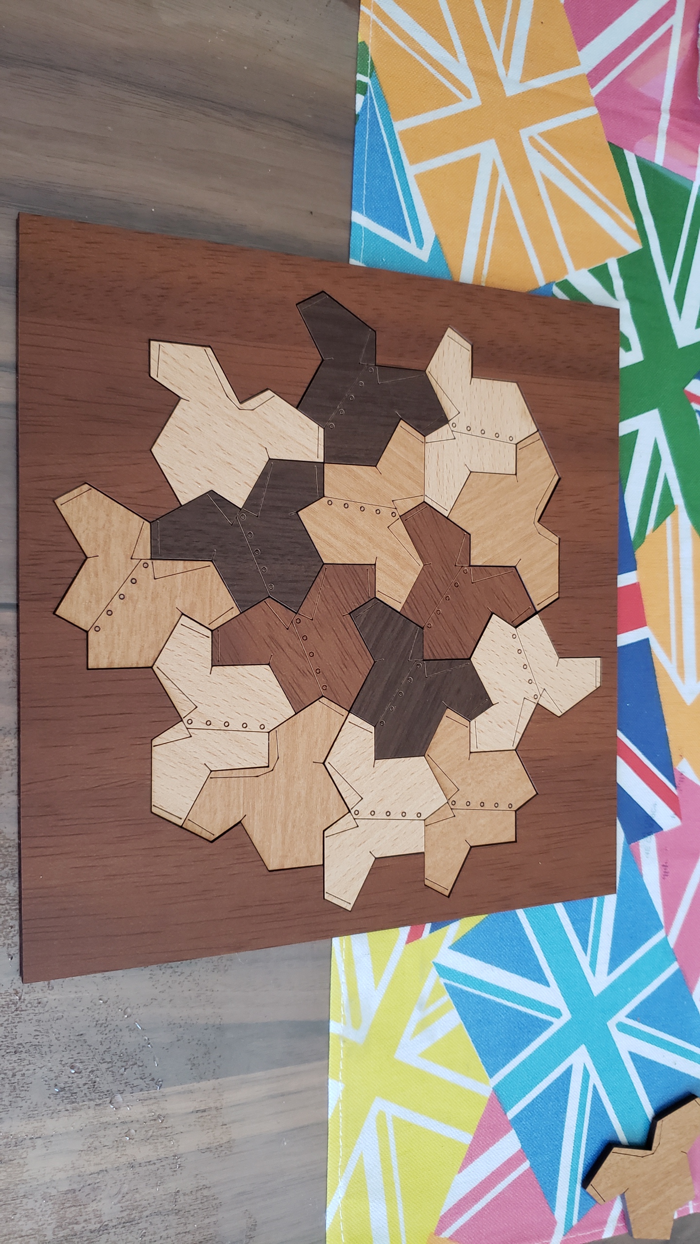
Everyone in the math community is all excited about the aperiodic monotiles that were discovered.
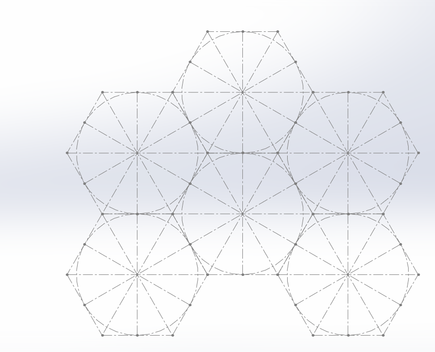
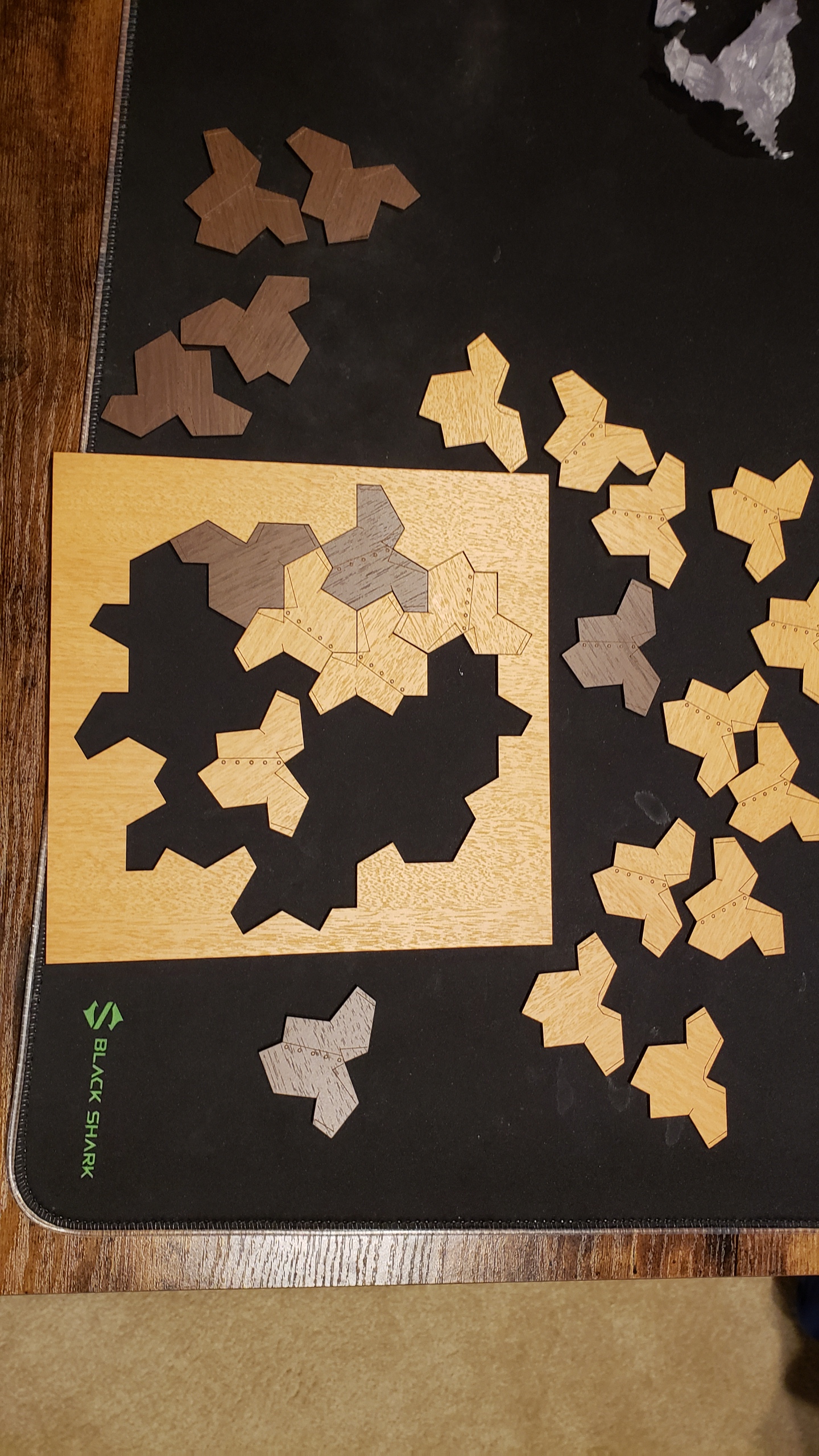
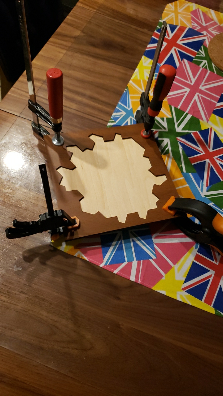
I don’t have much to add, but I did recreate it in Solidworks and laser cut it out:
I created a hexagon, and subdivided with construction lines, and saved that as a block.
I then inserted 5 more of these blocks:
Note that I think the ‘center’ doesn’t actually need to be in the center, and it will still tile, for more interesting shapes:
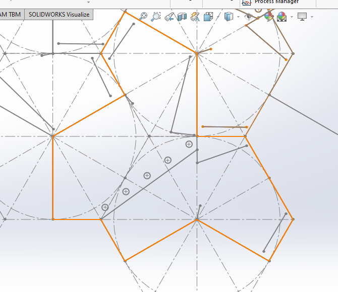
Then I draw the shape I wanted, shown in orange, and saved this as a block.
Then I created TWO new blocks. In the first block, I inserted that orange outline block, and drew on the shirt pattern. Then in the second block, I insert the same block, but mirrored it and drew on the back of the t-shirt.
Then I could insert a whole bunch of the two blocks, and manually arrange them together like a jigsaw, snapping edges together.
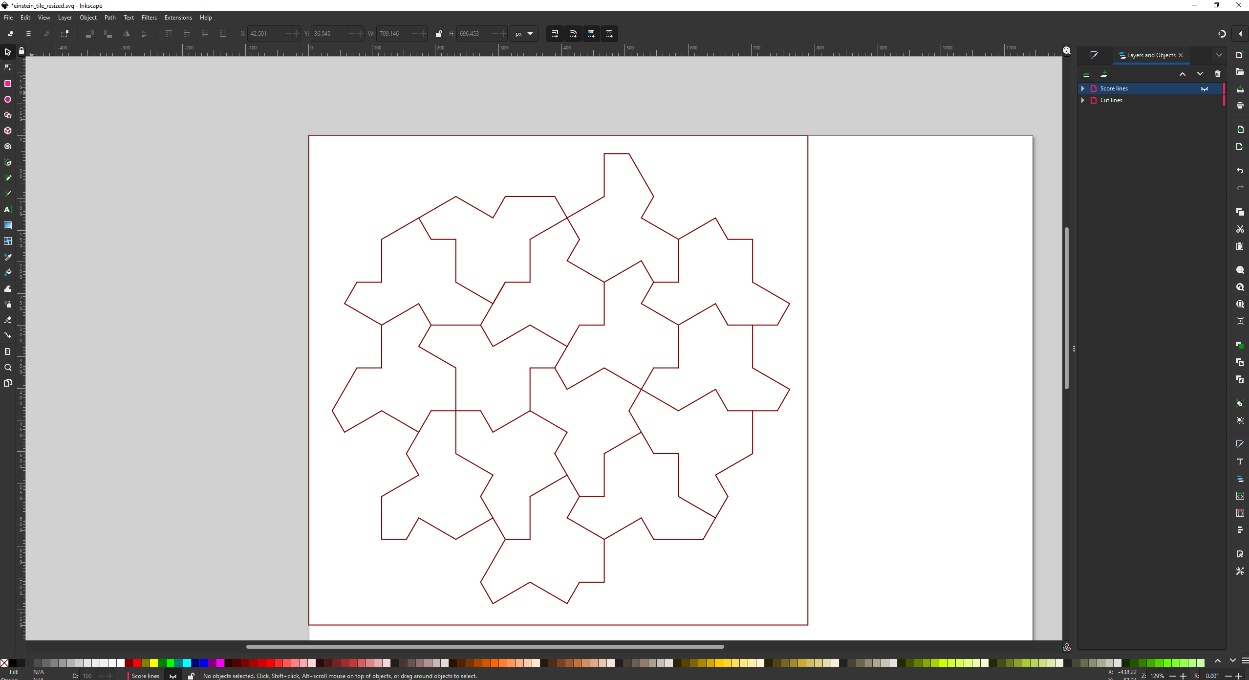
Then saved it as a DXF file and imported it into Inkscape, manually moving the cut lines and score lines to separate layers and giving them separate colors. I also had to manually delete overlapping lines. I’m not aware of a better approach.
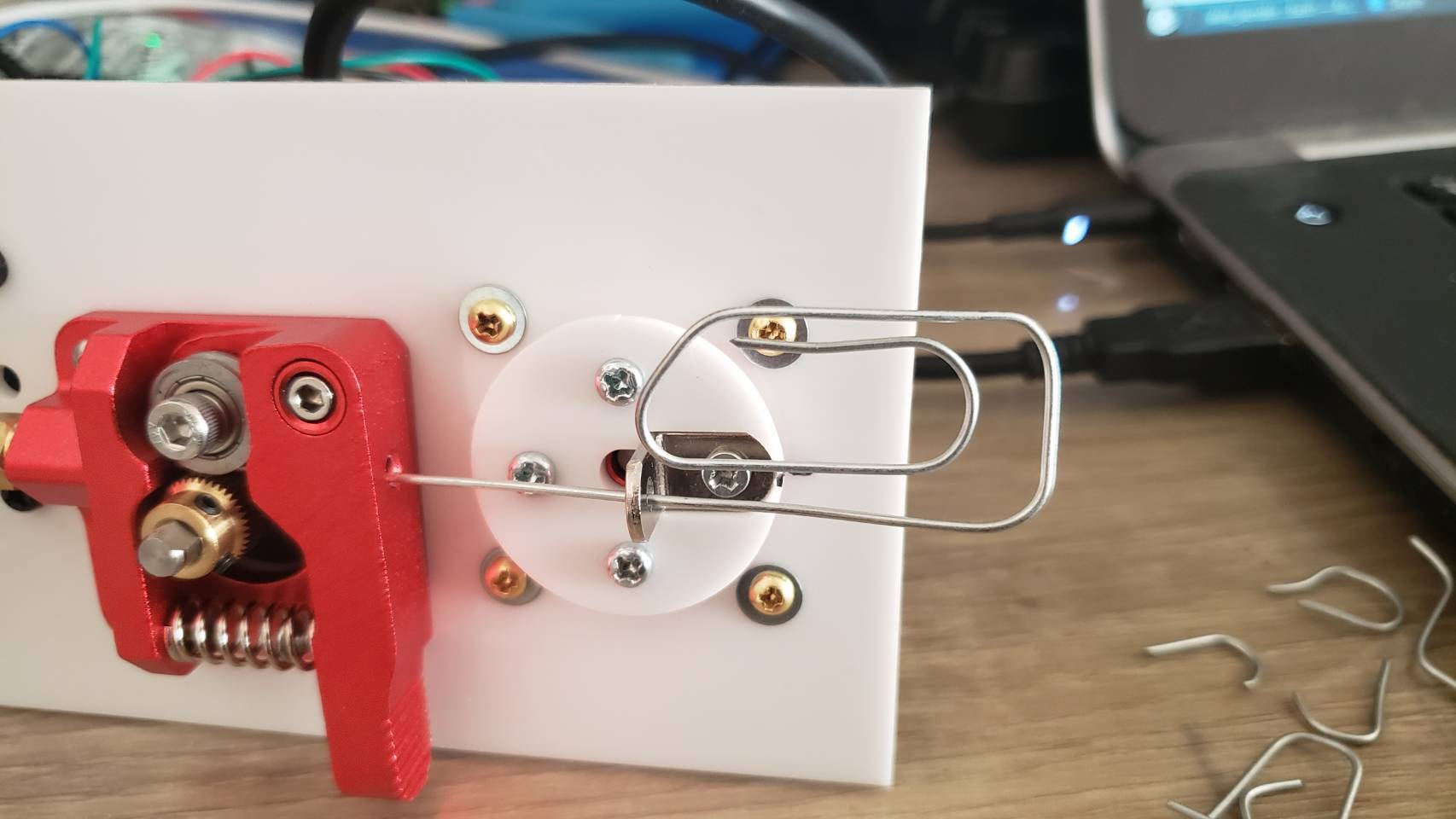
I wanted to bend a large amount of wire for another project.
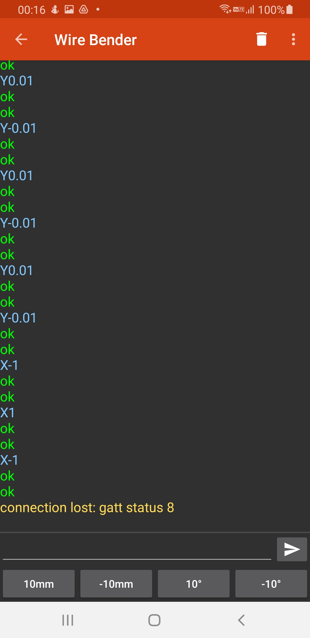
So I made this, a phone controlled wire bender. You plug it, establish a Bluetooth connection to it, and use the nifty android app I made to make it bend wire.
Details
I had an idea that an 3d printer’s extruder could also be used to extrude wire. So mocked something up:
And then laser cut it.
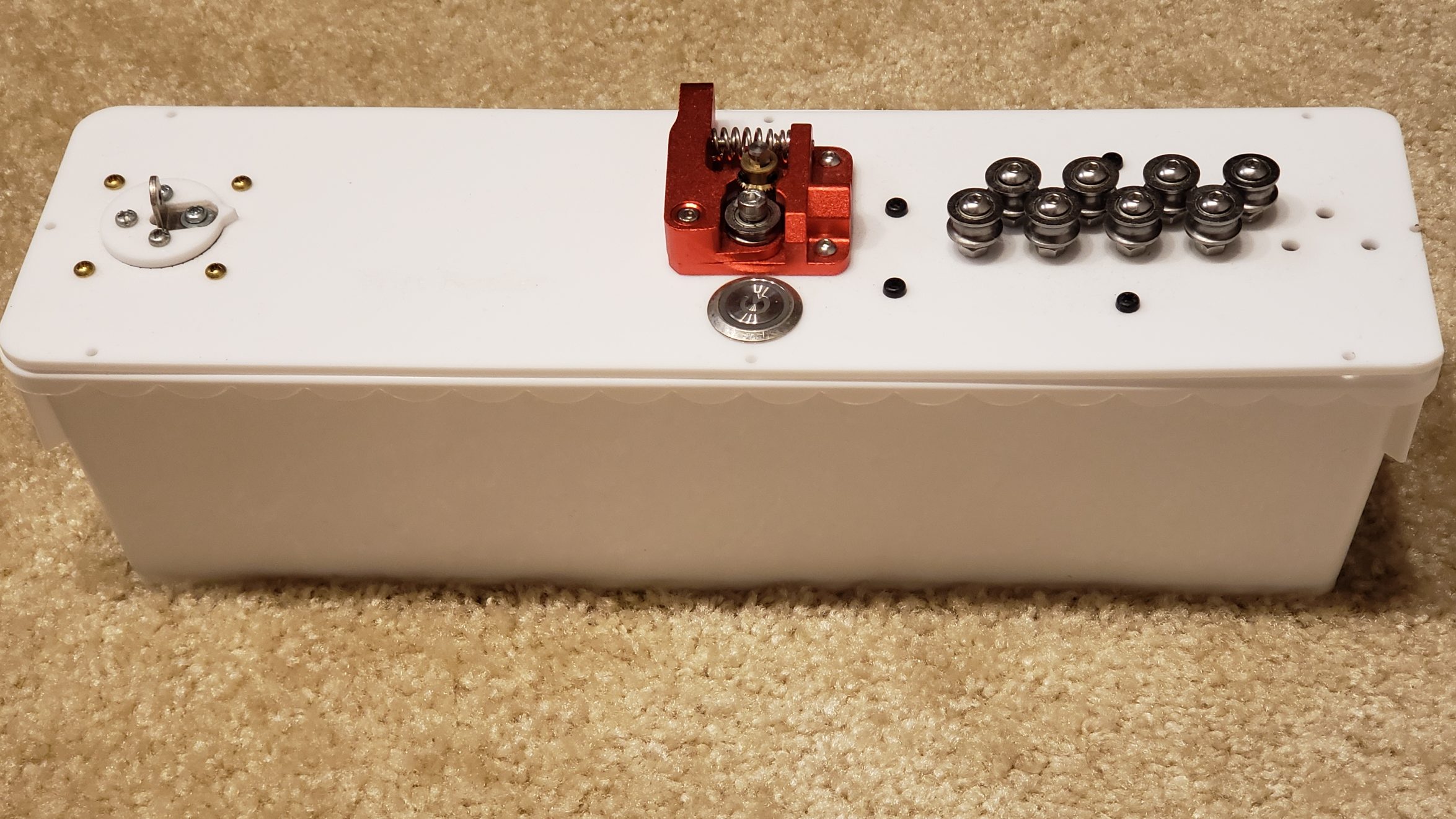
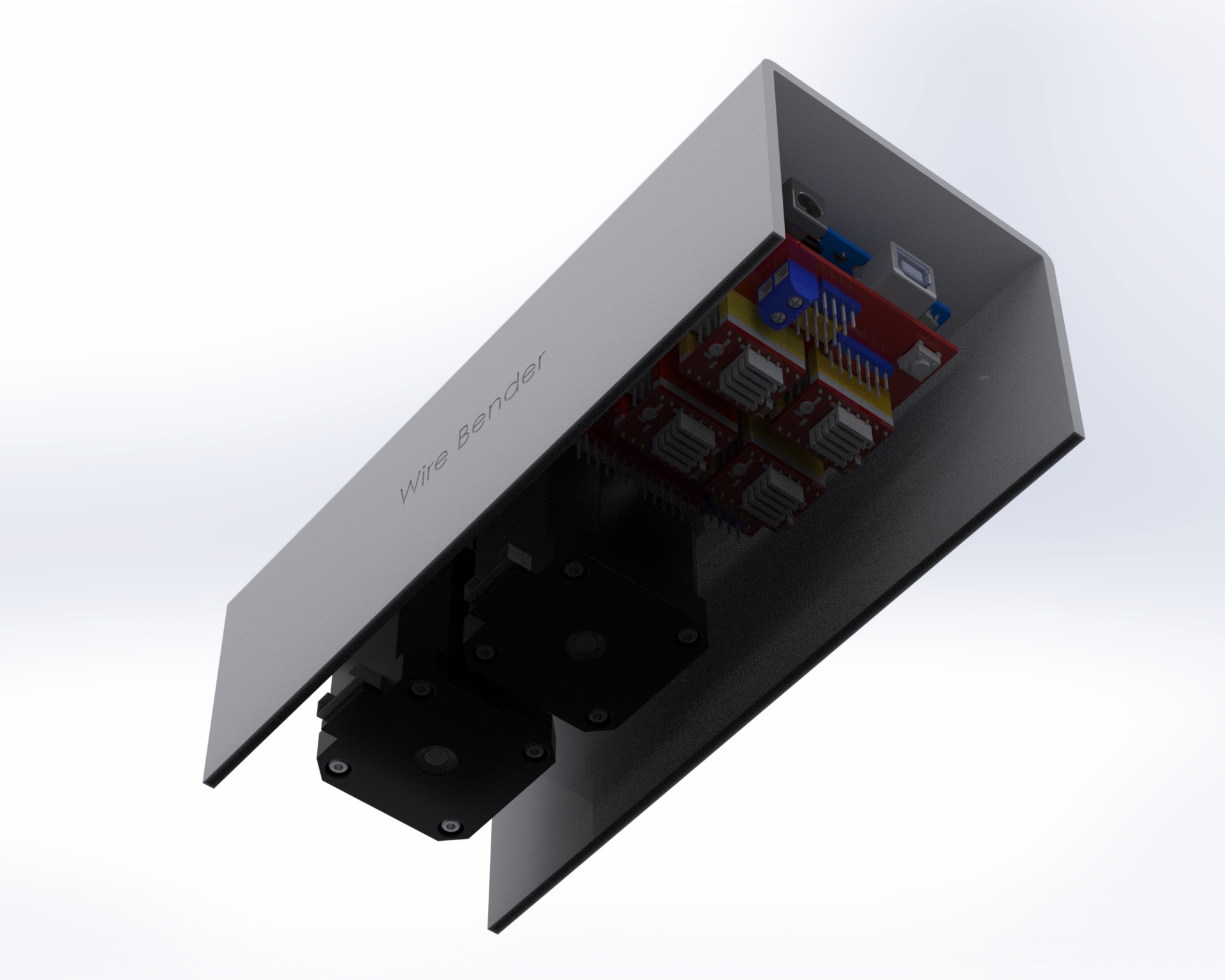
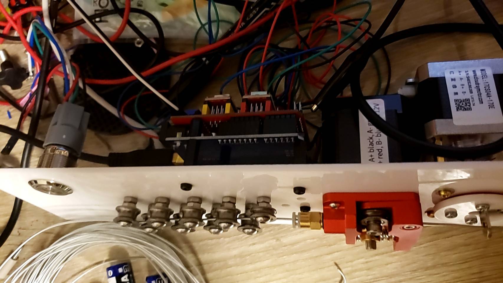
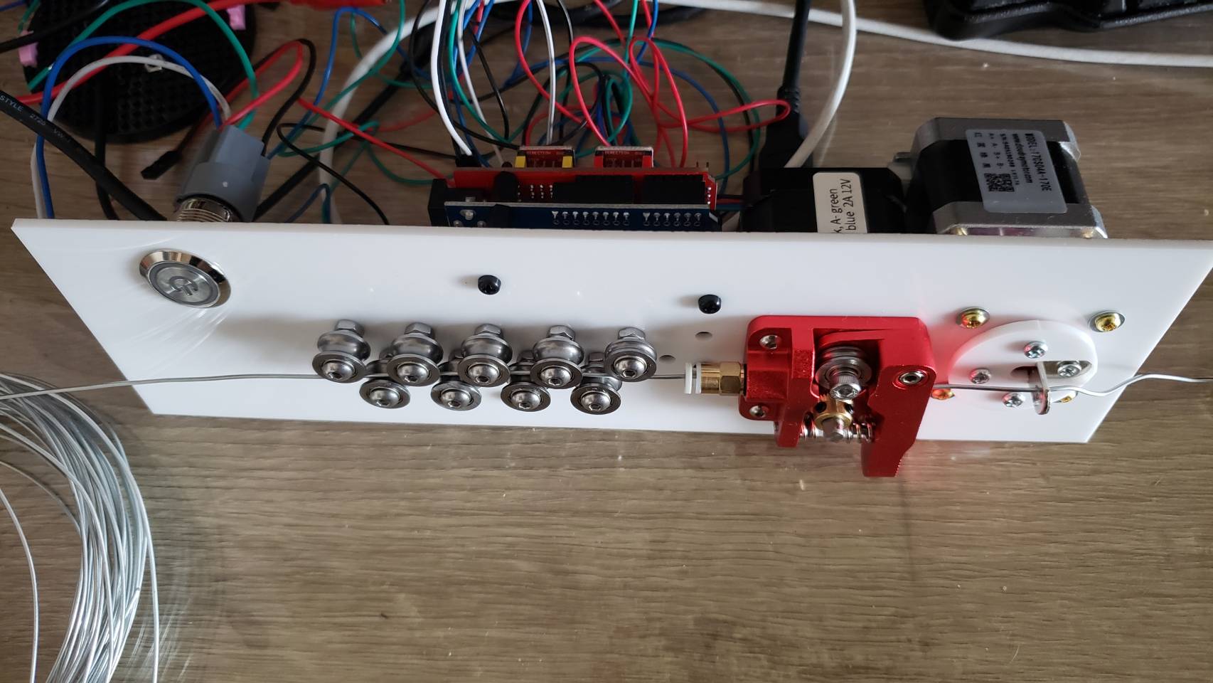
Mounting
I decided to mount everything to top acrylic, except for the power connector.
Also, I didn’t do much wire management 🙂
The “project box” is actually a flower pot 🙂
One thing I didn’t foresee with mounting everything upside down is that one of the heatsinks on the motor controller fell off. I had to add an acrylic plate on top to hold them in place. Also, I think I need some active cooling. I haven’t had any actual problems yet, despite bending a lot of wire, but I’m sure I’m doing the controllers and motors no favors.
Previous iterations
I actually went through quite a few iterations. Here was one of the first designs, before I realized that I needed the wire bending part to be much further away from the extruder:
I went through a few different iterations. The set of 11 feeder ball-bearings are there to straighten the wire. It’s not obvious, but they actually converge at approximately a 2 degree angle, and I find this works best. So when the wire is initially fed in, the large spaced bearings smooth out the large kinks, and then the closer spaced bearings smooth out the small kinks. Try trying to do it all in one pass doesn’t work because the friction ends up being too high.
I replaced the extruder feeder with one with a much more ‘grippy’ surface. The grooved metal needs to be harder than the wire you’re feeding into it, so that it can grip it well. This did result in marks in the metal, but that was okay for my purpose. Using two feeder motors could help with this.
Algorithm
The algorithm to turn an arbitrary shape into a set of motor controls was actually pretty interesting, and a large part of the project. Because you have to bend the wire further than the angle you actually want, because it springs back. I plan to write this part up properly later.
Software control
For computer control, I connect the stepper motors to a stepper motor driver, which I connect to an Arduino, which communicates over bluetooth serial to an android app. For prototyping I actually connected it to my laptop, and wrote a program in python to control it.
Both programs were pretty basic, but the android app has a lot more code for UI, bluetooth communication etc. The python code is lot easier to understand:
#!/usr/bin/env python3

import serial
import time
from termcolor import colored
from typing import Union
try:
    import gnureadline as readline
except ImportError:
    import readline

readline.parse_and_bind('tab: complete')
baud=9600 # We override Arduino/libraries/grbl/config.h to change to 9600
# because that's the default of the bluetooth module

try:
    s = serial.Serial('/dev/ttyUSB0',baud)
    print("Connected to /dev/ttyUSB0")
except:
    s = serial.Serial('/dev/ttyUSB1',baud)
    print("Connected to /dev/ttyUSB1")

# Wake up grbl
s.write(b"\r\n\r\n")
time.sleep(2)   # Wait for grbl to initialize
s.flushInput()  # Flush startup text in serial input

def readLineFromSerial():
    grbl_out: bytes = s.readline() # Wait for grbl response with carriage return
    print(colored(grbl_out.strip().decode('latin1'), 'green'))

def readAtLeastOneLineFromSerial():
    readLineFromSerial()
    while (s.inWaiting() > 0):
        readLineFromSerial()

def runCommand(cmd: Union[str, bytes]):
    if isinstance(cmd, str):
        cmd = cmd.encode('latin1')
    cmd = cmd.strip() # Strip all EOL characters for consistency
    print('>', cmd.decode('latin1'))
    s.write(cmd + b'\n') # Send g-code block to grbl
    readAtLeastOneLineFromSerial()

motor_angle: float = 0.0
MICROSTEPS: int = 16
YSCALE: float = 1000.0

def sign(x: float):
    return 1 if x >= 0 else -1

def motorYDeltaAngleToValue(delta_angle: float):
    return delta_angle / YSCALE

def motorXLengthToValue(delta_x: float):
    return delta_x

def rotateMotorY_noFeed(new_angle: float):
    global motor_angle
    delta_angle = new_angle - motor_angle
    runCommand(f"G1 Y{motorYDeltaAngleToValue(delta_angle):.3f}")
    motor_angle = new_angle

def rotateMotorY_feed(new_angle: float):
    global motor_angle
    delta_angle = new_angle - motor_angle
    motor_angle = new_angle
    Y = motorYDeltaAngleToValue(delta_angle)

    wire_bend_angle = 30 # fixme
    bend_radius = 3
    wire_length_needed = 3.1415 * bend_radius * bend_radius * wire_bend_angle / 360
    X = motorXLengthToValue(wire_length_needed)
    runCommand(f"G1 X{X:.3f} Y{Y:.3f}")

def rotateMotorY(new_angle: float):
    print(colored(f'{motor_angle}°→{new_angle}°', 'cyan'))
    if new_angle == motor_angle:
        return

    if sign(new_angle) != sign(motor_angle):
        # We are switching from one side to the other side.
        if abs(motor_angle) > 45:
            # First step is to move to 45 on the initial side, feeding the wire
            rotateMotorY_feed(sign(motor_angle) * 45)
        if abs(new_angle) > 45:
            rotateMotorY_noFeed(sign(new_angle) * 45)
            rotateMotorY_feed(new_angle)
        else:
            rotateMotorY_noFeed(new_angle)
    else:
        if abs(motor_angle) < 45 and abs(new_angle) < 45:
            # both start and end are less than 45, so no feeding needed
            rotateMotorY_noFeed(new_angle)
        elif abs(motor_angle) < 45:
            rotateMotorY_noFeed(sign(motor_angle) * 45)
            rotateMotorY_feed(new_angle)
        elif abs(new_angle) < 45:
            rotateMotorY_feed(sign(motor_angle) * 45)
            rotateMotorY_noFeed(new_angle)
        else: # both new and old angle are >45, so feed
            rotateMotorY_feed(new_angle)

def feed(delta_x: float):
    X = motorXLengthToValue(delta_x)
    runCommand(f"G1 X{X:.3f}")

def zigzag():
    for i in range(3):
        rotateMotorY(130)
        rotateMotorY(60)
        feed(5)
        rotateMotorY(0)
        feed(5)
        rotateMotorY(-130)
        rotateMotorY(-60)
        feed(5)
        rotateMotorY(0)
        feed(5)

def s_shape():
    for i in range(6):
        rotateMotorY(120)
        rotateMotorY(45)
    rotateMotorY(-130)
    for i in range(6):
        rotateMotorY(-120)
        rotateMotorY(-45)
    rotateMotorY(0)
    feed(20)

def paperclip():
    rotateMotorY(120)
    feed(1)
    rotateMotorY(130)
    rotateMotorY(140)

    rotateMotorY(30)
    feed(3)
    rotateMotorY(140)
    rotateMotorY(45)
    feed(4)
    feed(10)
    rotateMotorY(140)
    rotateMotorY(45)
    feed(3)
    rotateMotorY(140)
    rotateMotorY(50)
    rotateMotorY(150)
    rotateMotorY(45)
    feed(5)
    rotateMotorY(0)

runCommand('F32000') # Feed rate - affects X and Y
runCommand('G91')
runCommand('G21')  # millimeters
runCommand(f'$100={6.4375 * MICROSTEPS}') # Number of steps per mm for X
runCommand(f'$101={YSCALE * 0.5555 * MICROSTEPS}') # Number of steps per YSCALE degrees for Y
runCommand('?')
#rotateMotorY(-90)
#paperclip()
while True:
    line = input('> ("stop" to quit): ').upper()
    if line == 'STOP':
        break
    if len(line) == 0:
        continue
    cmd = line[0]
    if cmd == 'R':
        val = int(line[1:])
        rotateMotorY(val)
    elif cmd == 'F':
        val = int(line[1:])
        feed(val)
    else:
        runCommand(line)

runCommand('G4P0') # Wait for pending commands to finish
runCommand('?')

s.close()
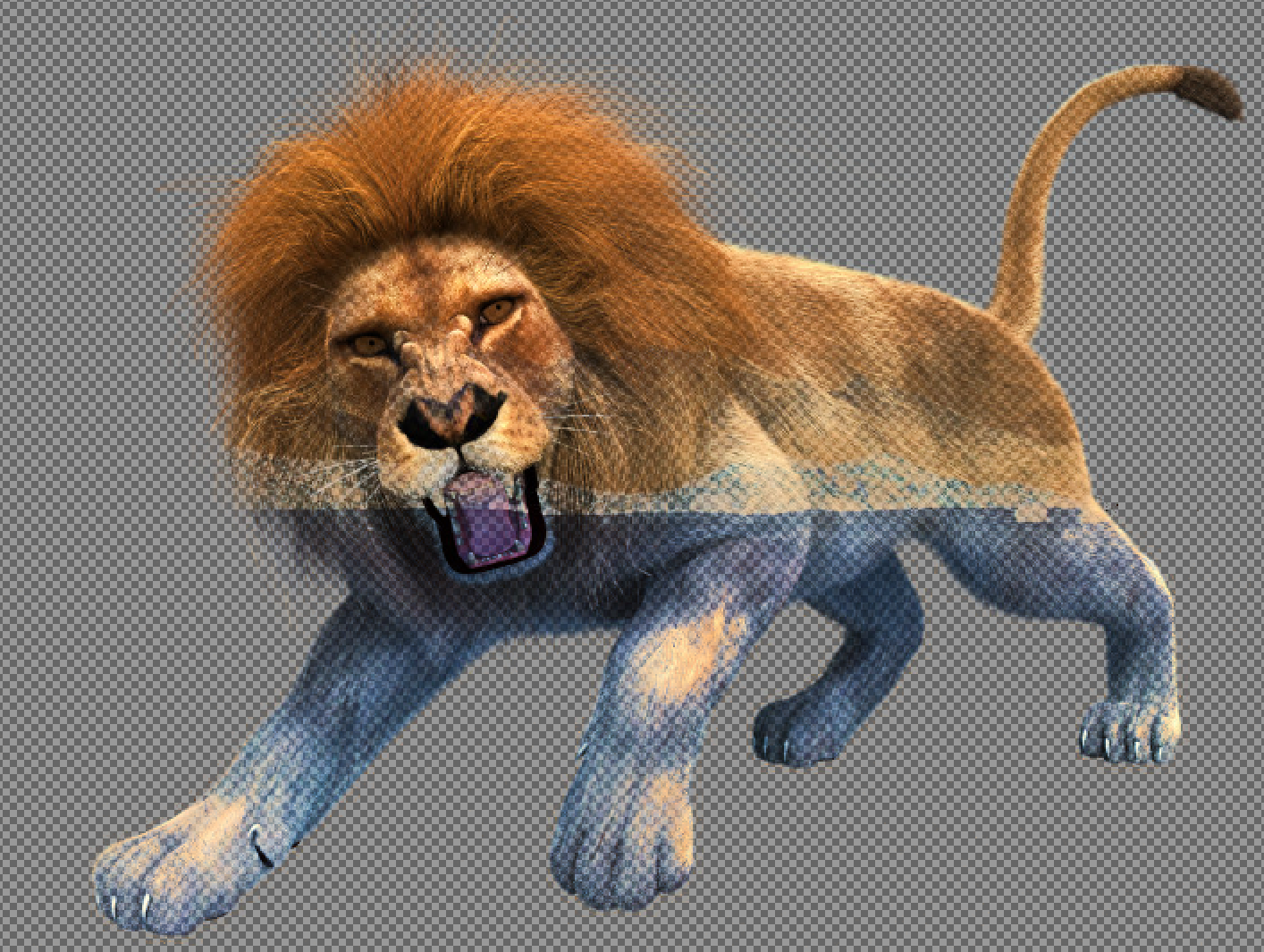
I have two opaque images – one with an object and a background, and another with just the background. Like:
Background
Background+foreground
I want to subtract the background from the image so that the alpha blended result is visually identical, but the foreground is as transparent as possible.
E.g:
Desired output (All images under Reuse With Modification license)
I’m sure that this must have been, but I couldn’t find a single correct way of doing this!
I asked a developer from the image editor gimp team, and they replied that the standard way is to create an alpha mask on the front image from the difference between the two images. i.e. for each pixel in both layers, subtract the rgb values, average that difference between the three channels, and then use that as an alpha.
But this is clearly not correct. Imagine the foreground has a green piece of semi-transparent glass against a red background. Just using an alpha mask is clearly not going to subtract the background because you need to actually modify the rgb values in the top layer image to remove all the red.
So what is the correct solution? Let’s do the calculations.
If we have a solution, the for a solid background with a semi-transparent foreground layer that is alpha blended on top, the final visual color is:
We want the visual result to be the same, so we know the value of – that’s our original foreground+background image. And we know – that’s our background image. We want to now create a new foreground image, , with the maximum value of .
So to restate this again – I want to know how to change the top layer so that I can have the maximum possible alpha without changing the final visual image at all. I.e. remove as much of the background as possible from our foreground+background image.
Note that we also have the constraint that for each color channel, that since each rgb pixel value is between 0 and 1. So:
So:
Proposal
Add an option for the gimp eraser tool to ‘remove layers underneath’, which grabs the rgb value of the layer underneath and applies the formula using the alpha in the brush as a normal erasure would, but bounding the alpha to be no more than the equation above, and modifying the rgb values accordingly.
Result
I showed this to the Gimp team, and they found a way to do this with the latest version in git. Open the two images as layers. For the top layer do: Layer->Transparency->Add Alpha Channel. Select the Clone tool. On the background layer, ctrl click anywhere to set the Clone source. In the Clone tool options, choose Default and Color erase, and set alignment to Registered. Make the size large, select the top layer again, and click on it to erase everything.
Result is:
When the background is a very different color, it works great – the sky was very nicely erased. But when the colors are too similar, it goes completely wrong.
This is a random idea that I’ve been thinking about. A reader messaged me to say that this look similar to online l-bgfs. To my inexperienced eyes, I can’t see this myself, but I’m still somewhat a beginner.
Yes, I chose a cat example simply so that I had an excuse to add cats to my blog.
Say we are training a neural network to take images of animals and classify the image as being an image of a cat or not a cat.
You would train the network to output, say, if the image is that of a cat.
To do so, we can gather some training data (images labelled by humans), and for each image we see what our network predicts (e.g. “I’m 40% sure it’s a cat”). We compare that against what a human says (“I’m 100% sure it’s a cat”) find the squared error (“We’re off by 0.6, so our squared error is 0.6^2”) and adjust each parameter, , in the network so that it slightly decreases the error (). And then repeat.
It’s this adjustment of each parameter that I want to rethink. The above procedure is Stochastic Gradient Descent (SGD) – we adjust to reduce the error for our test set (I’m glossing over overfitting, minibatches, etc).
Key Idea
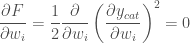
This means that we are also trying to look for a local minimum. i.e. that once trained, we want the property that if we varied any of the parameters by a small amount then it should increase the expected squared error
My idea is to encode this into the SGD update. To find a local minima for a particular test image we want:
(or if it equals 0, we need to consider the third differential etc).
Let’s concentrate on just the first criteria for the moment. Since we’ve already used the letter to mean the half squared error of , we’ll use to be the half squared error of .
So we want to minimize the half squared error :
So to minimize we need the gradient of this error:
Applying the chain rule:
SGD update rule
And so we can modify our SGD update rule to:
Where and are learning rate hyperparameters.
Conclusion
We finished with a new SGD update rule. I have no idea if this actually will be any better, and the only way to find out is to actually test. This is left as an exercise for the reader 😀
I wanted to find a best fit curve for some data points when I know that the true curve that I’m predicting is a parameter free Cumulative Distribution Function. I could just do a linear regression on the points, but the resulting function, might not have the properties that we desire from a CDF, such as:
Monotonically increasing
i.e. That it tends to 1 as x approaches positive infinity
i.e. That it tends to 0 as x approaches negative infinity
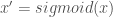
First, I take the second two points. To deal with this, I use the sigmoid function to create a new parameter, x’:
This has the nice property that and
So now we can find a best fit polynomial on .
So:
But with the boundary conditions that:
and
Which, solving for the boundary conditions, gives us:
Which simplifies our function to:
Implementing this in tensorflow using stochastic gradient descent (code is below) we get:
20 data samples
100 data samples
(The graph title equation is wrong. It should be then . I was too lazy to update the graphs sorry)
Unfortunately this curve doesn’t have one main property that we’d like – it’s not monotonically increasing – it goes above 1. I thought about it for a few hours and couldn’t think of a nice solution.
I’m sure all of this has been solved properly before, but with a quick google I couldn’t find anything.
Edit: I’m updating this 12 days later. I have been thinking in the background about how to enforce that I want my function to be monotonic. (i.e. always increasing/decreasing) I was certain that I was just being stupid and that there was a simple answer. But by complete coincidence, I watched the youtube video Breakthroughs in Machine Learning – Google I/O 2016 in which the last speaker mentioned this restriction. It turns out that this a very difficult problem – with the first solutions having a time complexity of :
I didn’t understand what exactly google’s solution for this is, but they reference their paper on it: Monotonic Calibrated Interpolated Look-up Tables, JMLR 2016. It seems that I have some light reading to do!
#!/usr/bin/env python
import tensorflow as tf
import numpy as np
import tensorflow as tf
import matplotlib.pyplot as plt
from scipy.stats import norm
# Create some random data as a binned normal function
plt.ion()
n_observations = 20
fig, ax = plt.subplots(1, 1)
xs = np.linspace(-3, 3, n_observations)
ys = norm.pdf(xs) * (1 + np.random.uniform(-1, 1, n_observations))
ys = np.cumsum(ys)
ax.scatter(xs, ys)
fig.show()
plt.draw()
highest_order_polynomial = 3
# We have our data now, so on with the tensorflow
# Setup the model graph
# Our input is an arbitrary number of data points (That's what the 'None dimension means)
# and each input has just a single value which is a float
X = tf.placeholder(tf.float32, [None])
Y = tf.placeholder(tf.float32, [None])
# Now, we know data fits a CDF function, so we know that
# ys(-inf) = 0 and ys(+inf) = 1
# So let's set:
X2 = tf.sigmoid(X)
# So now X2 is between [0,1]
# Let's now fit a polynomial like:
#
# Y = a + b*(X2) + c*(X2)^2 + d*(X2)^3 + .. + z(X2)^(highest_order_polynomial)
#
# to those points. But we know that since it's a CDF:
# Y(0) = 0 and y(1) = 1
#
# So solving for this:
# Y(0) = 0 = a
# b = (1-c-d-e-...-z)
#
# This simplifies our function to:
#
# y = (1-c-d-e-..-z)x + cx^2 + dx^3 + ex^4 .. + zx^(highest_order_polynomial)
#
# i.e. we have highest_order_polynomial-2 number of weights
W = tf.Variable(tf.zeros([highest_order_polynomial-1]))
# Now set up our equation:
Y_pred = tf.Variable(0.0)
b = (1 - tf.reduce_sum(W))
Y_pred = tf.add(Y_pred, b * tf.sigmoid(X2))
for n in xrange(2, highest_order_polynomial+1):
Y_pred = tf.add(Y_pred, tf.mul(tf.pow(X2, n), W[n-2]))
# Loss function measure the distance between our observations
# and predictions and average over them.
cost = tf.reduce_sum(tf.pow(Y_pred - Y, 2)) / (n_observations - 1)
# Regularization if we want it. Only needed if we have a large value for the highest_order_polynomial and are worried about overfitting
# It's also not clear to me if regularization is going to be doing what we want here
#cost = tf.add(cost, regularization_value * (b + tf.reduce_sum(W)))
# Use stochastic gradient descent to optimize W
# using adaptive learning rate
optimizer = tf.train.AdagradOptimizer(100.0).minimize(cost)
n_epochs = 10000
with tf.Session() as sess:
# Here we tell tensorflow that we want to initialize all
# the variables in the graph so we can use them
sess.run(tf.initialize_all_variables())
# Fit all training data
prev_training_cost = 0.0
for epoch_i in range(n_epochs):
sess.run(optimizer, feed_dict={X: xs, Y: ys})
training_cost = sess.run(
cost, feed_dict={X: xs, Y: ys})
if epoch_i % 100 == 0 or epoch_i == n_epochs-1:
print(training_cost)
# Allow the training to quit if we've reached a minimum
if np.abs(prev_training_cost - training_cost) &lt; 0.0000001:
break
prev_training_cost = training_cost
print "Training cost: ", training_cost, " after epoch:", epoch_i
w = W.eval()
b = 1 - np.sum(w)
equation = "x' = sigmoid(x), y = "+str(b)+"x' +" + (" + ".join("{}x'^{}".format(val, idx) for idx, val in enumerate(w, start=2))) + ")";
print "For function:", equation
pred_values = Y_pred.eval(feed_dict={X: xs}, session=sess)
ax.plot(xs, pred_values, 'r')
plt.title(equation)
fig.show()
plt.draw()
#ax.set_ylim([-3, 3])
plt.waitforbuttonpress()
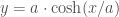
Now we have to decide how to cut the wood. To produce the arch, the angle of each piece of wood (the tangent lines), relative to the horizontal, is just: . So the angle between two adjacent pieces of wood is the difference between their angles.
The wood will be parallel with those tangent lines, so we can draw on the normal lines for those tangent lines, of the thickness of the wood:
def dy(x):
    '''return an approximation of dy/dx'''
    return (y(x+0.05) - y(x-0.05)) / 0.1

def normalAngle(x):
    if x == -L/2:
        return 0
    elif x == L/2:
        return math.pi
    return math.atan2(-1.0, dy(x));

WoodThickness = 50.0 # in millimeters

def getNormalCoords(x, ymidpoint, lineLength):
    tangent = dy(x)
    if tangent != 0:
        if x == -L/2 or x == L/2:
            normalSlope = 0
        else:
            normalSlope = -1 / dy(x)
        xlength = lineLength * math.cos(normalAngle(x))
        xstart = x-xlength/2
        xend = x+xlength/2
        ystart = ymidpoint + normalSlope * (xstart - x)
        yend = ymidpoint + normalSlope * (xend - x)
    else:
        xstart = x
        xend = x
        ystart = ymidpoint + lineLength/2
        yend = ymidpoint - lineLength/2
    return (xstart, ystart, xend, yend)

for block in blocks:
    (xstart, ystart, xend, yend) = getNormalCoords(block.midpoint_x, block.midpoint_y, WoodThickness)
    ax.plot([xstart, xend], [ystart, yend], 'b-', lw=1)
fig
Now, the red curve is going to represent the line of force. My reasoning is that if there was any force normal to the red curve, then the string/bridge/weight would thus accelerate and change position.
So to minimize the lateral forces where the wood meets, we want the wood cuts to be normal to the red line. We add that, then draw the whole block:
def getWoodCorners(block, x):
    ''' Return the top and bottom of the piece of wood whose cut passes through x,y(x), and whose middle is at xmid '''
    adjusted_thickness = WoodThickness / math.cos(normalAngle(x) - normalAngle(block.midpoint_x))
    return getNormalCoords(x, y(x), adjusted_thickness)

def drawPolygon(coords, linewidth):
    xcoords,ycoords = zip(*coords)
    xcoords = xcoords + (xcoords[0],)
    ycoords = ycoords + (ycoords[0],)
    ax.plot(xcoords, ycoords, 'k-', lw=linewidth)

#Draw all the blocks
for block in blocks:
    (xstart0, ystart0, xend0, yend0) = getWoodCorners(block, block.start_x) # Left side of block
    (xstart1, ystart1, xend1, yend1) = getWoodCorners(block, block.end_x) # Right side of block
    block.coords = [ (xstart0, ystart0), (xstart1, ystart1), (xend1, yend1), (xend0, yend0) ]
    drawPolygon(block.coords, 2) # Draw block

fig
There’s a few things to note here:
The code appears to do some pretty redundant calculations when calculating the angles – but much of this is to make the signs of the angles correct. It’s easier and nicer to let atan2 handle the signs for the quadrants, than to try to simplify the code and handle this ourselves.
The blocks aren’t actually exactly the same size at the points where they meet. The differences are on the order of 1%, and not noticeable in these drawings however.
Now we need to draw and label these blocks in a way that makes it easiest to cut:
fig, ax = subplots(1,1)
fig.set_size_inches(17,7)
axis('off')

def rotatePolygon(polygon,theta):
    """Rotates the given polygon which consists of corners represented as (x,y), around the ORIGIN, clock-wise, theta radians"""
    return [(x*math.cos(theta)-y*math.sin(theta) , x*math.sin(theta)+y*math.cos(theta)) for (x,y) in polygon]

def translatePolygon(polygon, xshift,yshift):
    """Shifts the polygon by the given amount"""
    return [ (x+xshift, y+yshift) for (x,y) in polygon]

sawThickness = 3.0 # add 3 mm gap between blocks for saw thickess
#Draw all the blocks
xshift = 10.0 # Start at 10mm to make it easier to cut by hand
topCutCoords = []
bottomCutCoords = []
for block in blocks:
    coords = translatePolygon(block.coords, -block.midpoint_x, -block.midpoint_y)
    coords = rotatePolygon(coords, -block.angle())
    coords = translatePolygon(coords, xshift - coords[0][0], -coords[3][1])
    xshift = coords[1][0] + sawThickness
    drawPolygon(coords,1)
    (topLeft, topRight, bottomRight, bottomLeft) = coords
    itopLeft = int(round(topLeft[0]))
    itopRight = int(round(topRight[0]))
    ibottomLeft = int(round(bottomLeft[0]))
    ibottomRight = int(round(bottomRight[0]))
    topCutCoords.append(itopLeft)
    topCutCoords.append(itopRight)
    bottomCutCoords.append(ibottomLeft)
    bottomCutCoords.append(ibottomRight)
    ax.text(topLeft[0], topLeft[1], itopLeft)
    ax.text(topRight[0], topRight[1], itopRight, horizontalalignment='right')
    ax.text(bottomLeft[0], bottomLeft[1], ibottomLeft, verticalalignment='top', horizontalalignment='center')
    ax.text(bottomRight[0], bottomRight[1], ibottomRight, verticalalignment='top', horizontalalignment='center')

print "Top coordinates:", topCutCoords
print "Bottom Coordinates:", bottomCutCoords
I wanted to have a modern aerodynamics simulator, to test out my flight control hardware and software.
Apologies in advance for a very terse post. I spent a lot of hours in a very short timespan to do this as a quick experiment.
So I used Unreal Engine 4 for the graphics engine, and built on top of that.
The main forces for a low speed aircraft that I want to model:
The lift force due to the wing
The drag force due to the wind
Gravity
Any horizontal forces from propellers in aircraft-style propulsion
Any vertical forces from propellers in quadcopter-style propulsion
Lift force due to the wing
The equation for the lift force is:
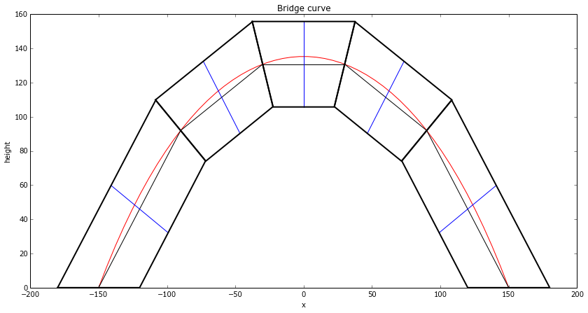
I created a function for the lift coefficient, , based on the angle, by calculating it theoretically. To get proper results, I would need to actually measure this in a wind tunnel, but this is good enough for a first approximation:
The horizontal axis is the angle of attack, in degrees. When the aircraft is flying “straight”, the angle of attack is not usually 0, but around 5 to 10 degrees, thus still providing an upward force.
I repeat this for each force in turn.
3D Model
To visualize it nicely, I modelled the craft in blender, manually set the texture space, and painted the texture in gimp. As you can tell from the texture space, there are several horrible problems with the geometry ‘loops’. But it took a whole day to get the top and bottom looking decent, and it was close enough for my purposes.
I imported the model into Unreal Engine 4, and used a high-resolution render for the version in the top right, and used a low-resolution version for the game.
Next, here’s the underneath view. You can see jagged edges in the model here, because at the time I didn’t understand how normal smoothing worked. After a quick google, I selected those vertexes in blender and enabled normal smoothing on them and fixed that.
and then finally, testing it out on the real thing:
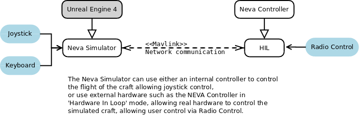
Architecture
The architecture is a fairly standard Hardware-in-loop system.
The key modules are:
The Flight Controller which controls the craft. This is not used if we are connected to external real hardware, such as the my controller.
The Communication Module to the real hardware, receiving information about the desired thrust of the engines and the Radio Control inputs from the user, and sending information about the current simulated position and speed.
The Physics Simulator which calculates the physical forces on the craft and applies them.
The User Interface which displays a lot of information about the craft as well as the internal controller.
The low level flight controller and network communication code is written in C++. Much of the high level logic is written in a visual language called ‘Blueprint’.
User Interface
From the GUI User Interface, you can control:
The aerodynamic forces on the wings
The height above ground to air pressure curve
The wing span and aerofoil chord length
The moment of inertia
The thrust of the turbines
The placement of the turbines
The PID values for the internal controller
Result
It worked pretty well.
It uses Hardware-In-Loop to allow the real hardware to control this, including a RC-Transmitter.
In this video I am allowing the PID algorithms to control the roll, pitch, yaw and height, which I then add to in order to control it.
PID Tuning
I implemented an auto-tuner for the PID algorithm, which you can tune and trigger from the GUI.
Hardware
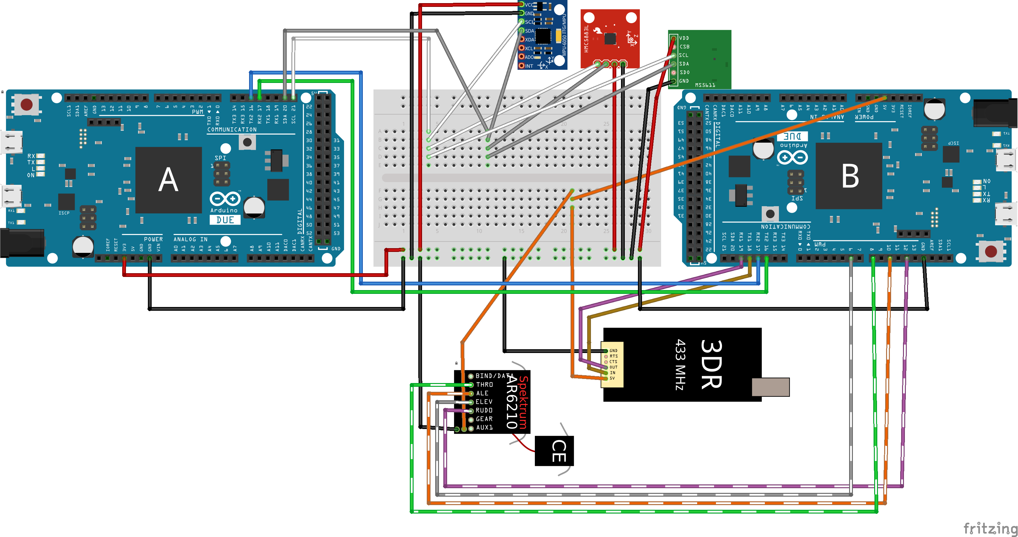
I used two arduinos to control the system:
And set up the Arduinos as so: (Btw, I used the Fritzing software for this – it’s pretty cool).
And putting together the hardware for testing (sorry for the mess). (I’m using QGroundControl to test it out).
And then mounting the hardware on a bit of wood as a base to keep it all together and make it more tidy:
I will hopefully later make a post about the software controlling this.
ESC Motor Controller Delay
I was particularly worried about the delay that the controller introduces.
I modified the program and used a basic UFO style quadcopter, then added in a 50ms buffer, to test the reaction.
For reference, here’s a photo of the real thing that I work on:
The quadcopter is programmed to try to hover over the chair.
I also tested with different latencies:
50ms really is the bare minimum that you can get away with.
These are manually tuned PIDs.
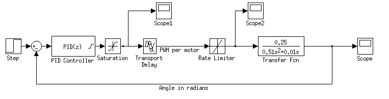
I did also simulate this system in 1D in Matlab’s Simulink:
A graph of the amplitude:
And finally, various bode plots etc. Just click on any for a larger image. Again, apologies for the awful terseness.
We need an AI that can play a perfect game of Snake. To collect the food without crashing into itself.
But it needs to run in real time on an 8Mhz processor, and use around 1 KB of memory. The extreme memory and speed restrictions means that we do not want to allocate any heap memory, and should run everything on the stack.
None of the conventional path finding algorithms would work here, so we need a new approach. The trick here is to realise that in the end part of the game, the snake will be following a planar Hamiltonian Cycle of a 2D array:
So what we can do is precompute a random hamiltonian cycle at the start of each game, then have the snake follow that cycle. It will thus pass through every point, without risk of crashing, and eventually win the game.
There are various way to create a hamiltonian cycle, but one way is to use Prim’s Algorithm to generate a maze of half the width and half the height. Then walk the maze by always turning left when possible. The resulting path will be twice the width and height and will be a hamiltonian cycle.
Now, we could have the snake just follow the cycle the entire time, but the result is very boring to watch because the snake does not follow the food, but instead just follows the preset path.
To solve this, I invented a new algorithm which I call the pertubated hamiltonian cycle. First, we imagine the cycle as being a 1D path. On this path we have the tail, the body, the head, and (wrapping back round again) the tail again.
The key is realising that as long as we always enforce this order, we won’t crash. As long as all parts of the body are between tail and the head, and as long as our snake does not grow long enough for the head to catch up with the tail, we will not crash.
This insight drastically simplifies the snake AI, because now we only need to worry about the position of the head and the tail, and we can trivially compute (in O(1)) the distance between the head and tail since that’s just the difference in position in the linear 1D array:
Now, this 1D array is actually embedded in a 2D array, and the head can actually move in any of 3 directions at any time. This is equivalent to taking shortcuts through the 1D array. If we want to stick to our conditions, then any shortcut must result in the head not overtaking the tail, and it shouldn’t overtake the food, if it hasn’t already. We must also leave sufficient room between the head and tail for the amount that we expect to grow.
Now we can use a standard shortest-path finding algorithm to find the optimal shortcut to the food. For example, an A* shortest path algorithm.
However I opted for the very simplest algorithm of just using a greedy search. It doesn’t produce an optimal path, but visually it was sufficiently good. I additionally disable the shortcuts when the snake takes up 50% of the board.
To test, I started with a simple non-random zig-zag cycle, but with shortcuts:
What you can see here is the snake following the zig-zag cycle, but occasionally taking shortcuts.
We can now switch to a random maze:
And once it’s working on the PC, get it working on the phone:
Code
NOTE: I have lost the original code, but I’ve recreated it and put it here:
This was my first electronics project – a simple self-balancing robot.
The wheels and chassis are from a toy truck. Onto that I salotaped a breadboard with two Light-Dependant-Resistors, attached in series. On one end I feed 5V, on the other end, ground. This gives a voltage divider. And in the middle I connect that to a resistor and a capacitor in parallel. This gives me a Proportional Derivative signal (out of a PID controller).
This means that we can read off the current ratio of brightness that the two LDRs see, then add on to that signal the rate at which they are changing. This helps prevent driving the motors too fast when we already moving rapidly towards the balancing point.
We then read this analog voltage on the Arduino, and use it to control the direction of the motors.
There is a huge amount of gear slop which is why it can only barely balance.


 – that’s our original foreground+background image. And we know
  – that’s our background image. We want to now create a new foreground image,
  , with the maximum value of
  .
. so that I can have the maximum possible alpha without changing the final visual image at all. I.e. remove as much of the background as possible from our foreground+background image.
 since each rgb pixel value is between 0 and 1. So:


 if the image is that of a cat.
 , in the network so that it slightly decreases the error (
 ). And then repeat.

 (or if it equals 0, we need to consider the third differential etc).
 , we’ll use
  to be the half squared error of
  .
.


 and
and  are learning rate hyperparameters.
 i.e. That it tends to 1 as x approaches positive infinity
 i.e. That it tends to 0 as x approaches negative infinity
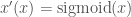
 and
and 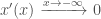
 .
.
 and
and 


 then
then  . I was too lazy to update the graphs sorry)
 :
:


 . So the angle between two adjacent pieces of wood is the difference between their angles.


 , based on the angle, by calculating it theoretically. To get proper results, I would need to actually measure this in a wind tunnel, but this is good enough for a first approximation:


")