I wanted a simple way to track the movement and orientation of an object (In this case, my Samurai robot). TrackIR’s SDK is not public, and has no python support as far as I know.
I looked at the symbols in dll that is distributed with the trackir app, and with some googling around on the function names, I could piece together how to use this API.
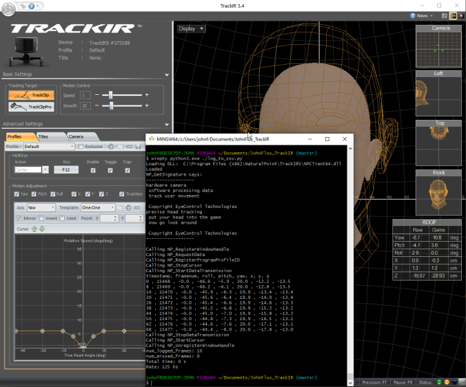
Here’s the result – my console program running in a window in the middle. I have pressed ctrl+c after 70ms, to cancel, to give a better screenshot:
Implementation Details
Python lets you call functions in any .dll library pretty easily (although the documentation for doing so is pretty awful). The entire code is approximately 500 lines, with half of that being comments, and I’ve put on github here:
Query the Windows registry for where the TrackIR software is installed.
Load the NPClient64.dll in that TrackIR software folder, using python ctypes.WinDLL (Note, I’m using 64 bit python, so I want the 64 bit library)
Expose each function in the dll that we want to use. This can get a bit cryptic, and took a bit of messing about to get right. For example, there is a function in the dll ‘NP_StopCursor’, that in C would look like:
where ‘NP_StopCursor’ is now a function that can then be called with: NP_StopCursor(). See the trackir.py file for more, including on how to pass parameters which are data structures etc.
Note: Python ctypes supports a way to mark a parameter as an ‘output’, but I didn’t fully understand what it was doing. It seemed to just work, and appeared to automatically allocate the memory for you, but the documentation didn’t explain it, and I didn’t entirely trust that I wasn’t just corrupting random memory, so I stuck to making all the parameters input parameters and ‘new’ing the data structure myself.
Create a graphical window and get its handle (hWnd), and call the functions in the TrackIR .dll to setup the polling, and pass the handle along. The TrackIR software will poll every 10 seconds ish to check that the given graphic window is still alive, and shutdown the connection if not.
Poll the DLL at 120hz to get the 6DOF position and orientation information.
ROS Integration
I wanted to get this to stream 6DOF data to ROS as well, to open up possibilities such as being able to determine the position of a robot, or to control the robot with your head etc.
The easiest way is to run a websocket server on the linux ROS server, and send the data via ROS message via the websocket.
I saw this for sale in a Christmas market for 500 yen (~$5 USD) and immediately bought it. My friends questioned my sanity, since it’s for “boy’s day” (It’s a “五月人形”) and we have no boys.
But, I could see the robotic potential!
Note: I have put the gold plated metal through an ultrasonic cleaner and buffed them with British Museum wax. But I’m not sure how to remove the corrosion – please message me if you have any ideas.
Next step is to build a wooden skeleton to mount the motors:
I’ve used 2 MG996 servo motors (presumably clones).
And a quick and dirty arduino program to move the head in a circular motion:
#include
Servo up_down_servo; // create servo object to control a servo
Servo left_right_servo; // create servo object to control a servo
int pos = 0; // variable to store the servo position
void setup() {
up_down_servo.attach(8); // attaches the servo on pin 8 to the servo object
up_down_servo.write(170); // Maximum is 170 and that's looking forward, and smallest is about 140 and that is looking a bit downwards
left_right_servo.attach(9); // attaches the servo on pin 9 to the servo object
left_right_servo.write(170); // 155 is facing forward. 170 is looking to the left for him
Serial.begin(115200);
Serial.println("up_down, left_right"); // Output a CSV stream, showing the desired positions
}
void loop() {
const float graduations = 1000.0;
for (pos = 0; pos < graduations; pos++) {
const float up_down_angle = 160+10*sin(pos / graduations * 2.0 * 3.1415);
const float left_right_angle = 155+5*cos(pos / graduations * 2.0 * 3.1415);
left_right_servo.write(left_right_angle);
up_down_servo.write(up_down_angle);
Serial.print(up_down_angle);
Serial.print(",");
Serial.println(left_right_angle);
delay(15);
}
}
And the result:
Jerky Movement
Unfortunately the movement of the head is extremely jerky. to quantify this, lets track the position accurately.
To do so, I mounted a TrackIR: 3 small reflective markers, which are then picked up by a camera. The position of the reflective markers are then determined, and the 6DOF position of the head calculated.
To actually log the data from TrackIR was tricky. To achieve this, I used FreePIE – an application for ‘bridging and emulating input devices’. It supports TrackIR as an input, and allows you to run a python function on input.
I wrote the following script to output CSV:
#Use Z to force flushing file to disk
import os
def update():
# Note that you need to set the
# curves for these to 1:1 in the TrackIR gui, which needs to be running
# at the same time.
yaw = trackIR.yaw
pitch = trackIR.pitch
roll = trackIR.roll
x = trackIR.x
y = trackIR.y
z = trackIR.z
csv_str = yaw.ToString() + "," + pitch.ToString() + "," + roll.ToString() + "," + x.ToString() + "," + y.ToString() + "," + z.ToString() + "\n"
#diagnostics.debug(csv_str)
f.write(csv_str)
if starting:
global f
trackIR.update += update
f = open("trackir output.csv","w")
diagnostics.debug("Logging to: " + os.path.realpath(f.name))
f.write("yaw,pitch,roll,x,y,z\n")
if keyboard.getPressed(Key.Z):
f.flush()
diagnostics.debug("flushing")
And taped the head tracker like so:
Note 1: I also set the TrackIR response curves to all be 1:1 and disabled smoothing of the input. We want the raw data. Although I later realised that freepie exposes the raw data, so I could have just used that instead.
Note 2: If you enable logging in FreePIE, it outputs the log to “C:\Program Files (x86)\FreePIE\trackirworker.txt”
Note 3: For some reason, FreePIE is only updating the TrackIR readings at 4hz. I don’t know why – I looked into the code, but without much success. I filed a bug.
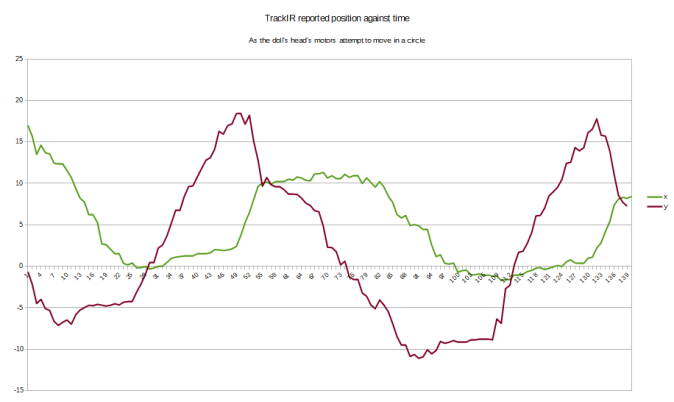
And here are the results:
There is a lot of a jerkiness here. This is supposed to look like a beautiful sinusoidal curve:
To fix this, and make the movement smooth, we need to understand where this jerkiness comes from.
Source of jerkiness
A quick word about motivation: For almost my entire life, I’ve wanted to build robots with smooth natural-looking movement, and I’ve hated the unnatural jerkiness that you often see.
A quick word about terminology: ‘Jerkiness’ has a real technical meaning – it is the function of position over time, differentiated 3 times. Since we are aiming for a circular movement, and since the 3rd order differential of a sinusoidal movement is still sinusoidal, even in the ideal situation there is still technically a non-zero jerk. So here I mean jerkiness in a more informal manor. I have previously written about, and written code for, motion planning with a guaranteed jerk of 0 when controlling a car, for which the jerkiness really must be minimized to prevent whiplash and discomfort.
We must understand how a servo works:
How a servo works
A servo is a small geared DC motor, a potentiometer to measure position, and a control circuit that presumably uses some basic PID algorithm to power the motor to try to match the potentiometer reading to the pulse width given on the input line:
To prevent the motor from ‘rocking’ back and forth around the desired value, the control circuit implements a ‘dead bandwith’ – a region in which it considers the current position to be ‘close enough’ to the given pulse.
For the MG996R servo that I’m using, the spec sheet says:
Note the ‘Dead band width’ of 5µs. The servo moves about 130 degrees when given a duty cycle between 800µs to 2200µs. NOTE: This means that the maximum duty cycle is only about 10% of the PWM period.
So this means that we move approximately 10µs per degree: (2200µs – 800µs)/130° ≈10µs.
So our dead band width is approximately 0.5°. Note that that means ±0.25°.
The arduino Servo::write(int angle) command takes an integer number of degrees, and by default is configured to 5µs per degree (2400µs – 544µs)/180° ≈10µs this means that we are introducing four times as much ‘jerkiness’ into our movement than we need to, simply from sloppy API usage. (Numbers taken from github Servo.h code)
So lets change the code to use the four times as accurate: Servo::writeMicroseconds(int microseconds) which lets us specify the number of microseconds for the duty cycle:
#include
Servo up_down_servo; // create servo object to control a servo
Servo left_right_servo; // create servo object to control a servo
int pos = 0; // variable to store the servo position
void servoAccurateWrite(const Servo &servo, float angle) {
/* 544 default used by Servo object, but ~800 on MG996R) */
const int min_duty_cycle_us = MIN_PULSE_WIDTH;
/* 2400 default used by Servo object, but ~2200 on MG996R) */
const int max_duty_cycle_us = MAX_PULSE_WIDTH;
/* Default used by Servo object, but ~130 on MG996R */
const int min_to_max_angle = 180;
const int duty_cycle_us = min + angle * (max - min)/min_to_max_angle;
servo.writeMicroseconds(duty_cycle_us);
}
void setup() {
up_down_servo.attach(8); // attaches the servo on pin 8 to the servo object
up_down_servo.write(170); // Maximum is 170 and that's looking forward, and smallest is about 140 and that is looking a bit downwards
left_right_servo.attach(9); // attaches the servo on pin 9 to the servo object
left_right_servo.write(170); // 155 is facing forward. 170 is looking to the left for him
Serial.begin(115200);
Serial.println("up_down, left_right"); // Output a CSV stream, showing the desired positions
}
void loop() {
const float graduations = 1000.0;
for (pos = 0; pos < graduations; pos++) {
const float up_down_angle = 160+10*sin(pos / graduations * 2.0 * 3.1415);
const float left_right_angle = 155+5*cos(pos / graduations * 2.0 * 3.1415);
servoAccurateWrite(left_right_servo, left_right_angle);
servoAccurateWrite(up_down_servo, up_down_angle);
Serial.print(up_down_angle);
Serial.print(",");
Serial.println(left_right_angle);
delay(15);
}
}
And the result of the position, as reported by TrackIR:
What a huge difference this makes! This is much more smooth. It doesn’t look very sinusoidal, but it’s a lot smoother.
Imagine you have a bluetooth device somewhere in your house, and you want to try to locate it. You have several other devices in the house that can see it, and so you want to triangulate its position.
This article is about the result I achieved, and the methodology.
I spent two solid weeks working on this, and this was the result:
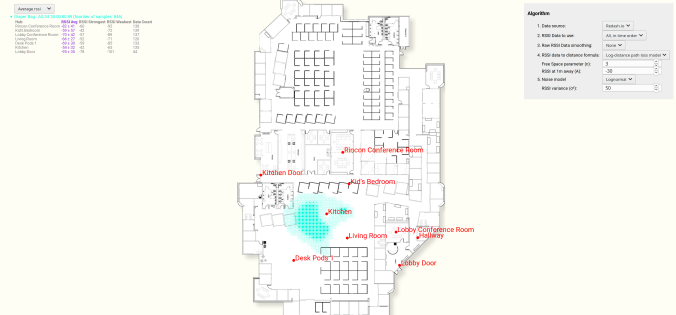
Estimating the most probable position of a bluetooth device, based on 7 strength readings.
We are seeing a map, overlaid in blue by the most likely position of a lost bluetooth device.
And a more advanced example, this time with many different devices, and a more advanced algorithm (discussed further below).
Note that some of the devices have very large uncertainties in their position.
Estimating position of multiple bluetooth devices, based on RSSI strength.
There are quite a few articles, video and books on estimating the distance of a bluetooth device (or wifi hub) based on knowing the RSSI signal strength readings.
But I couldn’t find any that gave the uncertainty of that estimation.
Noise is Normally distributed, with mean 0 and variance σ²
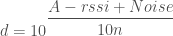
d is our distance (above) or estimated distance (below)
Rearranging to get an estimated distance, we get:
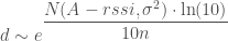
Now Noise is sampled from a Normal distribution, with mean = 0 and variance = σ², so let’s write our estimated d as a random variable:
Important note: Note that random variable d is distributed as the probability of the rssi given the distance. Not the probability of the distance given the rssi. This is important, and it means that we need to at least renormalize the probabilities over all possible distances to make sure that they add up to 1. See section at end for more details.
Adding a constant to a normal distribution just shifts the mean:
Now let’s have a bit of fun, by switching it to base e. This isn’t actually necessary, but it makes it straightforward to match up with wikipedia’s formulas later, so:
Distance in meters against probability density, for an rssi value of -80, A=-30, n=3, sigma^2=40
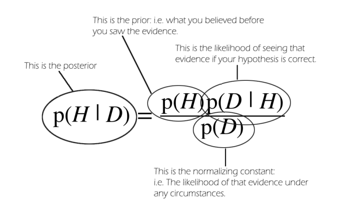
Bayes Theorem
I mentioned earlier:
Important note: Note that random variable d is distributed as the probability of the rssi given the distance. Not the probability of the distance given the rssi. This is important, and it means that we need to at least renormalize the probabilities over all possible distances to make sure that they add up to 1. See section at end for more details.
So using the above graph as an example, say that our measured RSSI was -80 and the probability density for d = 40 meters is 2%.


 is a
is a