For a client I needed a way to draw a gradient in realtime generated from four points, on a mobile phone. To produce an image like this, where the four gradient points can be moved in realtime:

I wanted to implement this using a shader, but after googling for a while I couldn’t find an existing implementation.
The problem is that I have the desired colours at four points, and need to calculate the colour at any other arbitrary point.
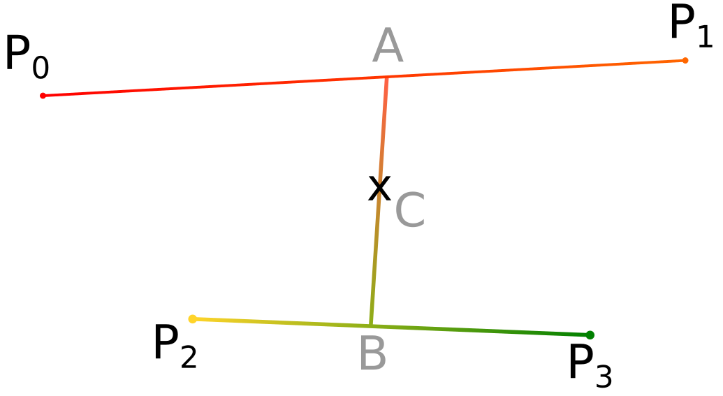
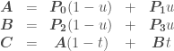
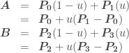
So we have three simultaneous equations (vectors in bold):

The key to solving this is to reduce the number of freedoms by setting  .
.
Solving for  gives us:

And solving for  and
and  :
:
so:

Defining:

Lets us now rewrite as:

Which written out for x and y is:

Now we have to consider the various different cases. If  then we have:

Likewise if 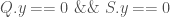 then we have:

Otherwise we are safe to divide by  and so:

Which can be solved with the quadratic formula when A is not zero: (Note that only the positive solution makes physical sense for us, and we can assume  )
)
and when A is zero (or, for computational rounding purposes, close to zero):

Math Summary
We can determine  and
and  with:
with:

Implementation as a shader:
This can be implemented as a shader as following: (The following can be run directly on https://www.shadertoy.com for example)
void mainImage( out vec4 fragColor, in vec2 fragCoord )
{

    //Example colors.  In practise these would be passed in
    // as parameters
    vec4 color0 = vec4(0.918, 0.824, 0.573, 1.0); // EAD292
    vec4 color1 = vec4(0.494, 0.694, 0.659, 1.0); // 7EB1A8
    vec4 color2 = vec4(0.992, 0.671, 0.537, 1.0); // FDAB89
    vec4 color3 = vec4(0.859, 0.047, 0.212, 1.0); // DB0C36

    vec2 uv = fragCoord.xy / iResolution.xy;

    //Example coordinates.  In practise these would be passed in
    // as parameters
    vec2 P0 = vec2(0.31,0.3);
    vec2 P1 = vec2(0.7,0.32);
    vec2 P2 = vec2(0.28,0.71);
    vec2 P3 = vec2(0.72,0.75);

    vec2 Q = P0 - P2;
    vec2 R = P1 - P0;
    vec2 S = R + P2 - P3;
    vec2 T = P0 - uv;

    float u;
    float t;

    if(Q.x == 0.0 && S.x == 0.0) {
        u = -T.x/R.x;
        t = (T.y + u*R.y) / (Q.y + u*S.y);
    } else if(Q.y == 0.0 && S.y == 0.0) {
        u = -T.y/R.y;
        t = (T.x + u*R.x) / (Q.x + u*S.x);
    } else {
        float A = S.x * R.y - R.x * S.y;
        float B = S.x * T.y - T.x * S.y + Q.x*R.y - R.x*Q.y;
        float C = Q.x * T.y - T.x * Q.y;
        // Solve Au^2 + Bu + C = 0
        if(abs(A) < 0.0001)
            u = -C/B;
        else
	    u = (-B+sqrt(B*B-4.0*A*C))/(2.0*A);
        t = (T.y + u*R.y) / (Q.y + u*S.y);
    }
    u = clamp(u,0.0,1.0);
    t = clamp(t,0.0,1.0);

    // These two lines smooth out t and u to avoid visual 'lines' at the boundaries.  They can be removed to improve performance at the cost of graphics quality.
    t = smoothstep(0.0, 1.0, t);
    u = smoothstep(0.0, 1.0, u);

    vec4 colorA = mix(color0,color1,u);
    vec4 colorB = mix(color2,color3,u);
    fragColor = mix(colorA, colorB, t);
}
And the same code again, but formatted as a more typical shader and with parameters:
uniform lowp vec4 color0;
uniform lowp vec4 color1;
uniform lowp vec4 color2;
uniform lowp vec4 color3;
uniform lowp vec2 p0;
uniform lowp vec2 p1;
uniform lowp vec2 p2;
uniform lowp vec2 p3;
varying lowp vec2 coord;
void main() {
lowp vec2 Q = p0 - p2;
lowp vec2 R = p1 - p0;
lowp vec2 S = R + p2 - p3;
lowp vec2 T = p0 - coord;
lowp float u;
lowp float t;
if(Q.x == 0.0 &amp;&amp; S.x == 0.0) {
u = -T.x/R.x;
t = (T.y + u*R.y) / (Q.y + u*S.y);
} else if(Q.y == 0.0 &amp;&amp; S.y == 0.0) {
u = -T.y/R.y;
t = (T.x + u*R.x) / (Q.x + u*S.x);
} else {
float A = S.x * R.y - R.x * S.y;
float B = S.x * T.y - T.x * S.y + Q.x*R.y - R.x*Q.y;
float C = Q.x * T.y - T.x * Q.y;
// Solve Au^2 + Bu + C = 0
if(abs(A) < 0.0001)
u = -C/B;
else
u = (-B+sqrt(B*B-4.0*A*C))/(2.0*A);
t = (T.y + u*R.y) / (Q.y + u*S.y);
}
u = clamp(u,0.0,1.0);
t = clamp(t,0.0,1.0);
// These two lines smooth out t and u to avoid visual 'lines' at the boundaries. They can be removed to improve performance at the cost of graphics quality.
t = smoothstep(0.0, 1.0, t);
u = smoothstep(0.0, 1.0, u);
lowp vec4 colorA = mix(color0,color1,u);
lowp vec4 colorB = mix(color2,color3,u);
gl_FragColor = mix(colorA, colorB, t);
}
Result
On the left is the result using smoothstep to smooth t and u, and on the right is the result without it. Although the non-linear smoothstep is computationally-expensive and a hack, I wasn’t happy with the visual lines that resulted in not using it.


 is a
is a 


 to
to  , and
, and  giving:

 “, but really it should be “Next two frequencies to add: … where
  ” since we are adding two frequencies at a time, in such a way that their imaginary parts cancel out, allowing us to keep everything real in the plots. I fixed this comment in the code, but didn’t want to rerender all the videos.
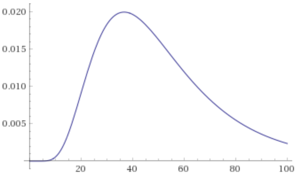
 . (A function that is 0 everywhere, except a sharp peak at exactly time = 0). In the S domain, this is a constant, meaning that we never converge. But visually it’s still cool.

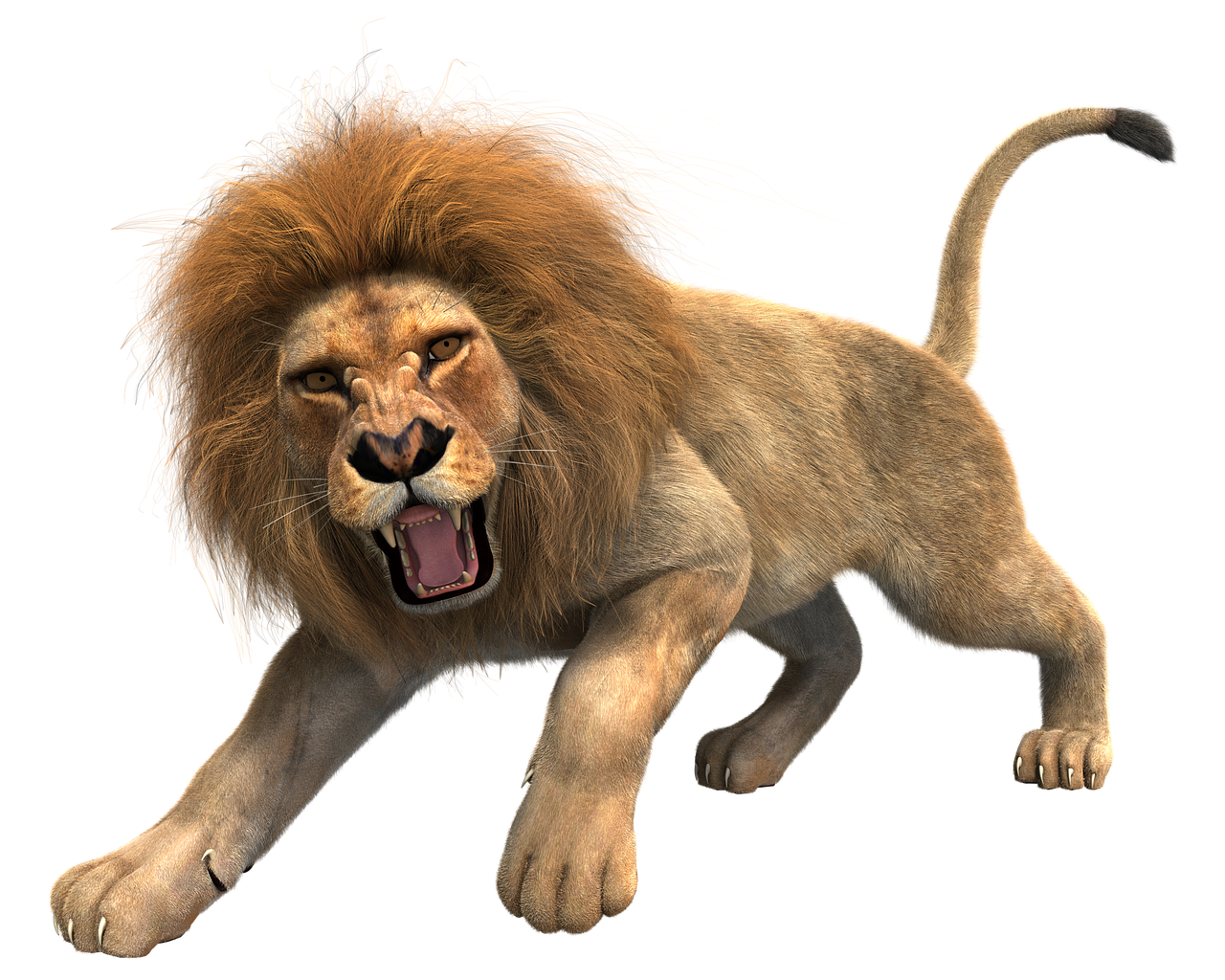

 – that’s our original foreground+background image. And we know
  – that’s our background image. We want to now create a new foreground image,
  , with the maximum value of
  .
. so that I can have the maximum possible alpha without changing the final visual image at all. I.e. remove as much of the background as possible from our foreground+background image.
 since each rgb pixel value is between 0 and 1. So:


 if the image is that of a cat.
 , in the network so that it slightly decreases the error (
 ). And then repeat.

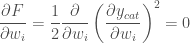
 (or if it equals 0, we need to consider the third differential etc).
 , we’ll use
  to be the half squared error of
  .
.


 and
and  are learning rate hyperparameters.
 i.e. That it tends to 1 as x approaches positive infinity
 i.e. That it tends to 0 as x approaches negative infinity
 and
and 
 .
.
 and
and 


 then
then  . I was too lazy to update the graphs sorry)
 :
:


