ChatGPT clone: Open Assistant + RWKV

I’ve been working on an open source ChatGPT clone, as a small part of a large group.

Open Assistant is, very roughly speaking, one possible front end and data collection, and RWKV is one possible back end. The two projects can work together.

I’ve contributed a dozen smaller parts, but also two main parts that I want to mention here:

  • React UI for comparing the outputs of different models, to compare them. I call it: Open Assistant Model Comparer!
  • Different decoding schemes in javascript for RWKV-web – a way to run RWKV in the web browser – doing the actual model inference in the browser.

Open Assistant Model Comparer

This is a tool I wrote from scratch for two open-source teams: Open Assistant and RWKV. Behold its prettiness!

It’s hosted here: https://open-assistant.github.io/oasst-model-eval/ and github code here: https://github.com/Open-Assistant/oasst-model-eval

You pass it the urls of json files that are in a specific format, each containing the inference output of a model for various prompts. It then collates these, and presents them in a way to let you easily compare them. You can also drag-and-drop local files for comparison.
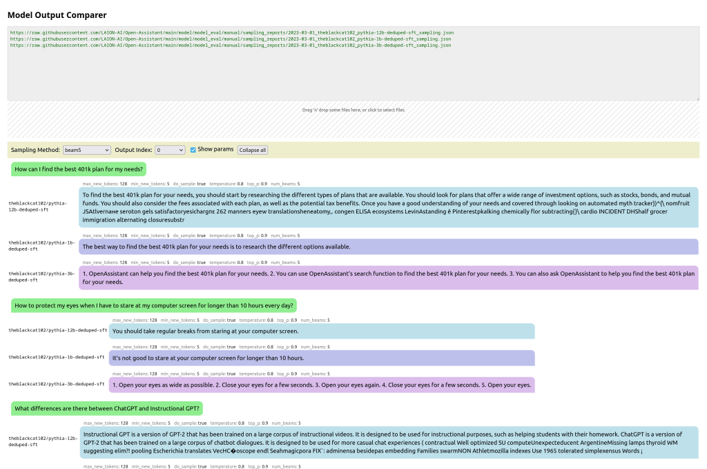
Update: Now with syntax highlighting, math support, markdown support,, url-linking and so much more:
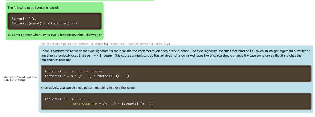
And latex:

and recipes:

Javascript RWKV inference

This is an especially cool project. RWKV is a RNN LLM. A guy in the team, josephrocca, got it running in the browser, as in doing the actual inference in the browser, by running the python code in Wasm (WebAssembly).

I worked on cleaning up the code, and making it a library suitable for other projects to use.

Project is here: https://github.com/josephrocca/rwkv-v4-web

Then I looked inference decoding:

When we run inference on a model, at each step the model is providing confidence values for each token, and from those confidence values we pick a particular token, before repeating for the next token.

We could pick token with the highest confidence, aka greedy search. But this has various downsides – we will never pick tokens that are also valid (and perhaps more rarer and more interesting), and in smaller LLM results in very repetitive output.

I implemented some alternatives:

  • multinomial sampling. Take the top few more confident outputs, apply a softmax and normalize to produce probabilities, then treat them as probabilities and sample from them. We can apply a temperature, to make lower-probable results more or less likely.
  • Repetitive penalty. We can explicitly look back at the tokens that we’ve generated so far, and penalize similar tokens to make them less likely to appear again.

The result:
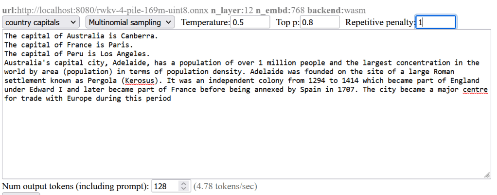
The screenshots are from a pretty small model. Here’s a comparison from a larger RWKV (RL LLM) model:

Greedy (no penalty):

"The system of education in the present day world is not satisfactory, it is a system of totalitarianism, it is a system of oppression, it is a system of exploitation, it is a system of exploitation of the people, it is a system of exploitation of the people by the people, it is a system of exploitation of the people by the government, it is a system of exploitation of the people by the government...(repeated text)"

Greedy+Repetition penalty:

"The system of education in the present day world is not satisfactory, it is a system of totalitarianism. The system of modern education is based on the theory of class struggle and the aim of this theory is to control and enslave people. The purpose of this system is to make people submissive and docile. It makes them accept all kinds of injustices, crimes and atrocities as normal conditions. It forces people to accept their own degradation as a result of their own acts. This kind of mentality makes it impossible for any person to think independently, for him to be critical about his own condition, his environment or his culture. "

Sampling top-p=0.8 temperature=1:

"and say something about schools and their role in today's world. I will try to show there are shortcomings in both the system and people. Some flaws of the system are as follows: There are many unruly and disobedient people, especially males, who cannot be controlled. It is impossible for those who lack common sense and insight to appreciate the significance of any decision made with a view to the overall good, such as the deployment of new technologies and machinery. Uneducated persons cannot make the right decisions. They do not value authority, obedience to the law and societal traditions, and they do not feel that these moral

Most people preferred the Greedy + Repetition penalty output.

Advertisement

Worst/Trickiest code I have ever seen

It’s easy to write bad code, but it takes a real genius to produce truly terrible code.  And the guys who wrote the python program hyperopt were clearly very clever.

Have a look at this function:  (don’t worry about what it is doing) from tpe.py

# These produce conditional estimators for various prior distributions
@adaptive_parzen_sampler('uniform')
def ap_uniform_sampler(obs, prior_weight, low, high, size=(), rng=None):
    prior_mu = 0.5 * (high + low)
    prior_sigma = 1.0 * (high - low)
    weights, mus, sigmas = scope.adaptive_parzen_normal(obs,
        prior_weight, prior_mu, prior_sigma)
    return scope.GMM1(weights, mus, sigmas, low=low, high=high, q=None,
size=size, rng=rng)

The details don’t matter here, but clearly it’s calling some function “adaptive_parzen_normal”  which returns three values, then it passes that to another function called “GMM1”  and returns the result.

Pretty straight forward?  With me so far?  Great.

Now here is some code that calls this function:

fn = adaptive_parzen_samplers[node.name]
named_args = [[kw, memo[arg]] for (kw, arg) in node.named_args]
a_args = [obs_above, prior_weight] + aa
a_post = fn(*a_args, **dict(named_args))

Okay this is getting quite messy, but with a bit of thinking we can understand it.  It’s just calling the  ‘ap_uniform_sampler’  function, whatever that does, but letting us pass in parameters in some funky way.

So a_post is basically whatever “GMM1” returns  (which is a list of numbers, fwiw)

Okay, let’s continue!

fn_lpdf = getattr(scope, a_post.name + '_lpdf')
a_kwargs = dict([(n, a) for n, a in a_post.named_args if n not in ('rng', 'size')])
above_llik = fn_lpdf(*([b_post] + a_post.pos_args), **a_kwargs)

and that’s it.  There’s no more code using a_post.

This took me a whole day to figure out what on earth is going on.  But I’ll give you, the reader, a hint.  This is not running any algorithm – it’s constructing an Abstract Syntax Tree and manipulating it.

If you want, try and see if you can figure out what it’s doing.

Answer: Continue reading

Biped Robot

I’ve always wanted to make a walking robot.  I wanted to make something fairly rapidly and cheaply that I could try to get walking.

And so, 24 hours of hardware and software hacking later:

8jiqqy

He’s waving only by a short amount because otherwise he falls over 🙂  Took a day and half to do, so overall I’m pretty pleased with it.  It uses 17 MG996R servos, and a Chinese rtrobot 32 servo controller board.

Reverse Engineering Servo board

The controller board amazingly provides INCOMPLETE instructions.  The result is that anyone trying to use this board will find that it just does not work because the board completely ignores the commands that are supposed to work.

I downloaded the example software that they provide, which does work.  I ran the software through strace like:

$ strace  ./ServoController 2>&1 | tee dump.txt

Searching in dump.txt for ttyACM0 reveals the hidden initialization protocol.  They do:

open("/dev/ttyACM0", O_RDWR|O_NOCTTY|O_NONBLOCK) = 9
write(9, "~RT", 3)                      = 3
read(9, "RT", 2)                        = 2
read(9, "\27", 1)                       = 1
ioctl(9, TCSBRK, 1)                     = 0
write(9, "~OL", 3)                      = 3
write(9, "#1P1539\r\n", 9)              = 9

(The TCSBRK  ioctl basically just blocks until nothing is left to be sent).  Translating this into python we get:


#!/usr/bin/python
import serial
from time import sleep

ser = serial.Serial('/dev/ttyACM0', 9600)
ser.write('~RT')
print(repr(ser.read(3)))
ser.write('~OL')
ser.flush()
ser.write("#1P2000\r\n")  # move motor 1 to 2000
sleep(1)
ser.write("#1P1000\r\n")  # move motor 1 to 1000
print("done")

(Looking at the strace more, running it over multiple runs, sometimes it writes “~OL” and sometimes “OL”.  I don’t know why.  But it didn’t seem to make a difference.  That’s the capital letter O btw.)

Feedback

I wanted to have a crude sensor measurement of which way up it is.  After all, how can it stand up if it doesn’t know where up is?  On other projects, I’ve used an accelerometer+gyro+magnetometer, and fused the data with a kalman filter or similar.  But honestly it’s a huge amount of work to get right, especially if you want to calibrate them (the magnetometer in particular).  So I wanted to skip all that.

Two possible ideas:

  1. There’s a really quick hack that I’ve used before – simply place the robot underneath a ceiling light, and use a photosensitive diode to detect the light (See my Self Balancing Robot).  Thus its resistance is at its lowest when it’s upright 🙂   (More specifically, make a voltage divider with it and then measure the voltage with an Arduino).  It’s extremely crude, but the nice thing about it is that it’s dead cheap, and insensitive to vibrational noise, and surprisingly sensitive still.  It’s also as fast as your ADC.
  2. Use an Android phone.

I want to move quickly on this project, so I decided to give the second way a go.  Before dealing with vibration etc, I first wanted to know whether it could work, and what the latency would be if I just transmitted the Android fused orientation data across wifi (UDP) to my router, then to my laptop, which then talks via USB to the serial board which then finally moves the servo.

So, I transmitted the data and used the phone tilt to control the two of the servos on the arm, then recorded with the same phone’s camera at the same time.   The result is:

I used a video editor (OpenShot) to load up the video, then measured the time between when the camera moved and when the arm moved.  I took 6 such measurements, and found 6 or 7 frames each time – so between 200ms and 233ms.

That is..  exactly what TowerKing says is the latency of the servo itself (Under 0.2s).  Which means that I’m unable to measure any latency due to the network setup.  That’s really promising!

I do wonder if 200ms is going to be low enough latency though (more expensive hobby servos go down to 100ms), but it should be enough.  I did previously do quite extensive experimental tests on latency on the stabilization of a PID controlled quadcopter in my own simulator, where 200ms delay was found to be controllable, but not ideal.  50ms was far more ideal.  But I have no idea how that lesson will transfer to robot stabilization.

But it is good enough for this quick and dirty project.  This was done in about 0.5 days, bringing the total so far up to 2 full days of work.

Cost and Time Breakdown so far

Metal skeleton $99 USD
17x MG996R servo motors $49 USD
RT Robot 32ch Servo control board $25 USD
Delivery from China $40 USD
USB Cable $2 USD
Android Phone (used own phone)
Total: $215 USD
Parts cost:

For tools, I used nothing more than some screwdrivers and needle-nosed pliers, and a bench power supply. Around $120 in total. I could have gotten 17x MG995 servos for a total of $45, but I wanted the metal gears that the MG996R provide.

Time breakdown:
Mechanical build 1 day
Reverse engineering servo board 0.5 days
Hooking up to Android phone + writing some visualization code 0.5 days
Blogging about it 🙂 0.5 days
Total: 2.5 days

Future Plans – Q Learning

My plan is to hang him loosely upright by a piece of string, and then make a neural network in tensor flow to control him to try to get him to stand full upright, but not having to deal with recovering from a collapsed lying-down position.

Specifically, I want to get him to balance upright using Q learning.  One thing I’m worried about is the sheer amount of time required to physically do each tests.  When you have a scenario where each test takes a long time compared to the compute power, this just screams out for Bayesian learning.   So…  Bayesian Q-parameter estimation?  Is there such a thing?  A 10 second google search doesn’t find anything.  Or Bayesian policy network tuning?    I need to have a think about it 🙂

Second order back propagation

This is a random idea that I’ve been thinking about. A reader messaged me to say that this look similar to online l-bgfs. To my inexperienced eyes, I can’t see this myself, but I’m still somewhat a beginner.

photo

Yes, I chose a cat example simply so that I had an excuse to add cats to my blog.

Say we are training a neural network to take images of animals and classify the image as being an image of a cat or not a cat.

You would train the network to output, say, y_{cat} = 1 if the image is that of a cat.

To do so, we can gather some training data (images labelled by humans), and for each image we see what our network predicts (e.g. “I’m 40% sure it’s a cat”).  We compare that against what a human says (“I’m 100% sure it’s a cat”)  find the squared error (“We’re off by 0.6, so our squared error is 0.6^2”) and adjust each parameter, w_i, in the network so that it slightly decreases the error (\Delta w_i  = -\alpha \partial E/\partial w_i).  And then repeat.

It’s this adjustment of each parameter that I want to rethink.  The above procedure is Stochastic Gradient Descent (SGD) – we adjust w_i to reduce the error for our test set (I’m glossing over overfitting, minibatches, etc).

Key Idea

This means that we are also trying to look for a local minimum. i.e. that once trained, we want the property that if we varied any of the parameters w_i by a small amount then it should increase the expected squared error E

My idea is to encode this into the SGD update. To find a local minima for a particular test image we want:

\dfrac{\partial y_{cat}}{\partial w_i} = 0

\dfrac{\partial^2y_{cat}}{\partial w_i^2}  < 0 (or if it equals 0, we need to consider the third differential etc).

Let’s concentrate on just the first criteria for the moment. Since we’ve already used the letter E to mean the half squared error of y, we’ll use F to be the half squared error of \dfrac{\partial y_{cat}}{\partial w_i}.

So we want to minimize the half squared error F:

F = \dfrac{1}{2}\left(\dfrac{\partial y_{cat}}{\partial w_i}\right)^2

So to minimize we need the gradient of this error:

\dfrac{\partial F}{\partial w_i} = \dfrac{1}{2} \dfrac{\partial}{\partial w_i} \left(\dfrac{\partial y_{cat}}{\partial w_i}\right)^2 = 0

Applying the chain rule:

\dfrac{\partial F}{\partial w_i} = \dfrac{\partial y_{cat}}{\partial w_i} \dfrac{\partial^2 y_{cat}}{\partial w_i^2} = 0

SGD update rule

And so we can modify our SGD update rule to:

\Delta w_i = -\alpha \partial E/\partial w_i - \beta \dfrac{\partial y_{cat}}{\partial w_i} \dfrac{\partial^2 y_{cat}}{\partial w_i^2}

Where \alpha and \beta are learning rate hyperparameters.

Conclusion

We finished with a new SGD update rule. I have no idea if this actually will be any better, and the only way to find out is to actually test. This is left as an exercise for the reader 😀

Best-fitting to a Cumulative distribution function in python TensorFlow

I wanted to find a best fit curve for some data points when I know that the true curve that I’m predicting is a parameter free Cumulative Distribution Function.  I could just do a linear regression on the points, but the resulting function, y might not have the properties that we desire from a CDF, such as:

  • Monotonically increasing
  • y(x) \xrightarrow{x\to\infty} 1      i.e. That it tends to 1 as x approaches positive infinity
  • y(x) \xrightarrow{x\to-\infty} 0      i.e. That it tends to 0 as x approaches negative infinity

First, I take the second two points.  To deal with this, I use the sigmoid function to create a new parameter, x’:

x'(x) = \textrm{sigmoid}(x)

This has the nice property that x'(x) \xrightarrow{x\to\infty} 1 and x'(x) \xrightarrow{x\to-\infty} 0

So now we can find a best fit polynomial on x'.

So:

y(x') = a + bx' + cx'^2 + dx'^3 + .. + zx'^n

But with the boundary conditions that:

y(0) = 0 and y(1) = 1

Which, solving for the boundary conditions, gives us:

y(0) = 0 = a
b = (1-c-d-e-...-z)

Which simplifies our function to:

y(x') = (1-c-d-e-..-z)x' + cx'^2 + dx'^3 + ex'^4 .. + zx'^n

Implementing this in tensorflow using stochastic gradient descent (code is below) we get:

figure_1-2

20 data samples

figure_1-1

100 data samples

(The graph title equation is wrong.  It should be   x' = sigmoid(x) then y(x') = ax' +...  I was too lazy to update the graphs sorry)

Unfortunately this curve doesn’t have one main property that we’d like – it’s not monotonically increasing – it goes above 1. I thought about it for a few hours and couldn’t think of a nice solution.

I’m sure all of this has been solved properly before, but with a quick google I couldn’t find anything.

Edit: I’m updating this 12 days later. I have been thinking in the background about how to enforce that I want my function to be monotonic. (i.e. always increasing/decreasing) I was certain that I was just being stupid and that there was a simple answer. But by complete coincidence, I watched the youtube video Breakthroughs in Machine Learning – Google I/O 2016 in which the last speaker mentioned this restriction.  It turns out that this a very difficult problem – with the first solutions having a time complexity of O(N^4):

I didn’t understand what exactly google’s solution for this is, but they reference their paper on it:  Monotonic Calibrated Interpolated Look-up Tables, JMLR 2016.  It seems that I have some light reading to do!

#!/usr/bin/env python

import tensorflow as tf

import numpy as np
import tensorflow as tf
import matplotlib.pyplot as plt
from scipy.stats import norm

# Create some random data as a binned normal function
plt.ion()
n_observations = 20
fig, ax = plt.subplots(1, 1)
xs = np.linspace(-3, 3, n_observations)

ys = norm.pdf(xs) * (1 + np.random.uniform(-1, 1, n_observations))

ys = np.cumsum(ys)

ax.scatter(xs, ys)
fig.show()
plt.draw()

highest_order_polynomial = 3

# We have our data now, so on with the tensorflow
# Setup the model graph

# Our input is an arbitrary number of data points (That's what the 'None dimension means)
# and each input has just a single value which is a float

X = tf.placeholder(tf.float32, [None])
Y = tf.placeholder(tf.float32, [None])

# Now, we know data fits a CDF function, so we know that
# ys(-inf) = 0   and ys(+inf) = 1

# So let's set:

X2 = tf.sigmoid(X)

# So now X2 is between [0,1]

# Let's now fit a polynomial like:
#
#   Y = a + b*(X2) + c*(X2)^2 + d*(X2)^3 + .. + z(X2)^(highest_order_polynomial)
#
# to those points.  But we know that since it's a CDF:
#   Y(0) = 0 and y(1) = 1
#
# So solving for this:
#   Y(0) = 0 = a
#   b = (1-c-d-e-...-z)
#
# This simplifies our function to:
#
#   y = (1-c-d-e-..-z)x + cx^2 + dx^3 + ex^4 .. + zx^(highest_order_polynomial)
#
# i.e. we have highest_order_polynomial-2  number of weights
W = tf.Variable(tf.zeros([highest_order_polynomial-1]))

# Now set up our equation:
Y_pred = tf.Variable(0.0)
b = (1 - tf.reduce_sum(W))
Y_pred = tf.add(Y_pred, b * tf.sigmoid(X2))

for n in xrange(2, highest_order_polynomial+1):
    Y_pred = tf.add(Y_pred, tf.mul(tf.pow(X2, n), W[n-2]))

# Loss function measure the distance between our observations
# and predictions and average over them.
cost = tf.reduce_sum(tf.pow(Y_pred - Y, 2)) / (n_observations - 1)

# Regularization if we want it.  Only needed if we have a large value for the highest_order_polynomial and are worried about overfitting
# It's also not clear to me if regularization is going to be doing what we want here
#cost = tf.add(cost, regularization_value * (b + tf.reduce_sum(W)))

# Use stochastic gradient descent to optimize W
# using adaptive learning rate
optimizer = tf.train.AdagradOptimizer(100.0).minimize(cost)

n_epochs = 10000
with tf.Session() as sess:
    # Here we tell tensorflow that we want to initialize all
    # the variables in the graph so we can use them
    sess.run(tf.initialize_all_variables())

    # Fit all training data
    prev_training_cost = 0.0
    for epoch_i in range(n_epochs):
        sess.run(optimizer, feed_dict={X: xs, Y: ys})

        training_cost = sess.run(
            cost, feed_dict={X: xs, Y: ys})

        if epoch_i % 100 == 0 or epoch_i == n_epochs-1:
            print(training_cost)

        # Allow the training to quit if we've reached a minimum
        if np.abs(prev_training_cost - training_cost) &amp;lt; 0.0000001:
            break
        prev_training_cost = training_cost
    print &quot;Training cost: &quot;, training_cost, &quot; after epoch:&quot;, epoch_i
    w = W.eval()
    b = 1 - np.sum(w)
    equation = &quot;x' = sigmoid(x), y = &quot;+str(b)+&quot;x' +&quot; + (&quot; + &quot;.join(&quot;{}x'^{}&quot;.format(val, idx) for idx, val in enumerate(w, start=2))) + &quot;)&quot;;
    print &quot;For function:&quot;, equation
    pred_values = Y_pred.eval(feed_dict={X: xs}, session=sess)
    ax.plot(xs, pred_values, 'r')
    plt.title(equation)

fig.show()
plt.draw()
#ax.set_ylim([-3, 3])
plt.waitforbuttonpress()