I wanted to find a best fit curve for some data points when I know that the true curve that I’m predicting is a parameter free Cumulative Distribution Function.  I could just do a linear regression on the points, but the resulting function, might not have the properties that we desire from a CDF, such as:

• Monotonically increasing
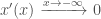
•      i.e. That it tends to 1 as x approaches positive infinity
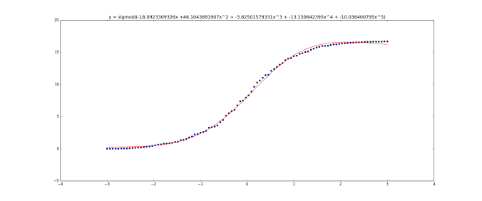
•      i.e. That it tends to 0 as x approaches negative infinity

First, I take the second two points.  To deal with this, I use the sigmoid function to create a new parameter, x’:

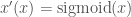
This has the nice property that and

So now we can find a best fit polynomial on .

So:

But with the boundary conditions that:

and

Which, solving for the boundary conditions, gives us:

Which simplifies our function to:

Implementing this in tensorflow using stochastic gradient descent (code is below) we get:

(The graph title equation is wrong.  It should be 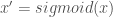  then .  I was too lazy to update the graphs sorry)

Unfortunately this curve doesn’t have one main property that we’d like – it’s not monotonically increasing – it goes above 1. I thought about it for a few hours and couldn’t think of a nice solution.

I’m sure all of this has been solved properly before, but with a quick google I couldn’t find anything.

Edit: I’m updating this 12 days later. I have been thinking in the background about how to enforce that I want my function to be monotonic. (i.e. always increasing/decreasing) I was certain that I was just being stupid and that there was a simple answer. But by complete coincidence, I watched the youtube video Breakthroughs in Machine Learning – Google I/O 2016 in which the last speaker mentioned this restriction.  It turns out that this a very difficult problem – with the first solutions having a time complexity of :

I didn’t understand what exactly google’s solution for this is, but they reference their paper on it:  Monotonic Calibrated Interpolated Look-up Tables, JMLR 2016.  It seems that I have some light reading to do!

#!/usr/bin/env python

import tensorflow as tf

import numpy as np
import tensorflow as tf
import matplotlib.pyplot as plt
from scipy.stats import norm

# Create some random data as a binned normal function
plt.ion()
n_observations = 20
fig, ax = plt.subplots(1, 1)
xs = np.linspace(-3, 3, n_observations)

ys = norm.pdf(xs) * (1 + np.random.uniform(-1, 1, n_observations))

ys = np.cumsum(ys)

ax.scatter(xs, ys)
fig.show()
plt.draw()

highest_order_polynomial = 3

# We have our data now, so on with the tensorflow
# Setup the model graph

# Our input is an arbitrary number of data points (That's what the 'None dimension means)
# and each input has just a single value which is a float

X = tf.placeholder(tf.float32, [None])
Y = tf.placeholder(tf.float32, [None])

# Now, we know data fits a CDF function, so we know that
# ys(-inf) = 0   and ys(+inf) = 1

# So let's set:

X2 = tf.sigmoid(X)

# So now X2 is between [0,1]

# Let's now fit a polynomial like:
#
#   Y = a + b*(X2) + c*(X2)^2 + d*(X2)^3 + .. + z(X2)^(highest_order_polynomial)
#
# to those points.  But we know that since it's a CDF:
#   Y(0) = 0 and y(1) = 1
#
# So solving for this:
#   Y(0) = 0 = a
#   b = (1-c-d-e-...-z)
#
# This simplifies our function to:
#
#   y = (1-c-d-e-..-z)x + cx^2 + dx^3 + ex^4 .. + zx^(highest_order_polynomial)
#
# i.e. we have highest_order_polynomial-2  number of weights
W = tf.Variable(tf.zeros([highest_order_polynomial-1]))

# Now set up our equation:
Y_pred = tf.Variable(0.0)
b = (1 - tf.reduce_sum(W))
Y_pred = tf.add(Y_pred, b * tf.sigmoid(X2))

for n in xrange(2, highest_order_polynomial+1):
    Y_pred = tf.add(Y_pred, tf.mul(tf.pow(X2, n), W[n-2]))

# Loss function measure the distance between our observations
# and predictions and average over them.
cost = tf.reduce_sum(tf.pow(Y_pred - Y, 2)) / (n_observations - 1)

# Regularization if we want it.  Only needed if we have a large value for the highest_order_polynomial and are worried about overfitting
# It's also not clear to me if regularization is going to be doing what we want here
#cost = tf.add(cost, regularization_value * (b + tf.reduce_sum(W)))

# Use stochastic gradient descent to optimize W
# using adaptive learning rate
optimizer = tf.train.AdagradOptimizer(100.0).minimize(cost)

n_epochs = 10000
with tf.Session() as sess:
    # Here we tell tensorflow that we want to initialize all
    # the variables in the graph so we can use them
    sess.run(tf.initialize_all_variables())

    # Fit all training data
    prev_training_cost = 0.0
    for epoch_i in range(n_epochs):
        sess.run(optimizer, feed_dict={X: xs, Y: ys})

        training_cost = sess.run(
            cost, feed_dict={X: xs, Y: ys})

        if epoch_i % 100 == 0 or epoch_i == n_epochs-1:
            print(training_cost)

        # Allow the training to quit if we've reached a minimum
        if np.abs(prev_training_cost - training_cost) < 0.0000001:
            break
        prev_training_cost = training_cost
    print "Training cost: ", training_cost, " after epoch:", epoch_i
    w = W.eval()
    b = 1 - np.sum(w)
    equation = "x' = sigmoid(x), y = "+str(b)+"x' +" + (" + ".join("{}x'^{}".format(val, idx) for idx, val in enumerate(w, start=2))) + ")";
    print "For function:", equation
    pred_values = Y_pred.eval(feed_dict={X: xs}, session=sess)
    ax.plot(xs, pred_values, 'r')
    plt.title(equation)

fig.show()
plt.draw()
#ax.set_ylim([-3, 3])
plt.waitforbuttonpress()