Imagine you have a bluetooth device somewhere in your house, and you want to try to locate it. You have several other devices in the house that can see it, and so you want to triangulate its position.
This article is about the result I achieved, and the methodology.
I spent two solid weeks working on this, and this was the result:
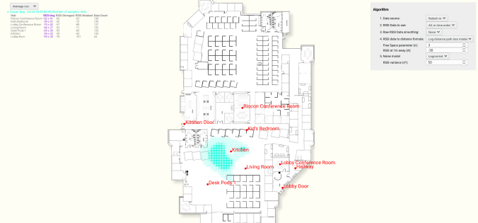
Estimating the most probable position of a bluetooth device, based on 7 strength readings.
We are seeing a map, overlaid in blue by the most likely position of a lost bluetooth device.
And a more advanced example, this time with many different devices, and a more advanced algorithm (discussed further below).
Note that some of the devices have very large uncertainties in their position.

Estimating position of multiple bluetooth devices, based on RSSI strength.
And to tie it all together, a mobile app:

Methodology
There are quite a few articles, video and books on estimating the distance of a bluetooth device (or wifi hub) based on knowing the RSSI signal strength readings.
But I couldn’t find any that gave the uncertainty of that estimation.
So here I derive it myself, using the Log-distance_path loss model

In this model:
- rssi is the signal strength, measured in dB
- n is a ‘path loss exponent’:

- A is the rssi value at 1 meter away
- Noise is Normally distributed, with mean 0 and variance σ²
- d is our distance (above) or estimated distance (below)
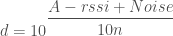

Important note: Note that random variable d is distributed as the probability of the rssi given the distance. Not the probability of the distance given the rssi. This is important, and it means that we need to at least renormalize the probabilities over all possible distances to make sure that they add up to 1. See section at end for more details.

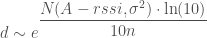

 is a Lognormal distribution:


Distance in meters against probability density, for an rssi value of -80, A=-30, n=3, sigma^2=40
Bayes Theorem
I mentioned earlier:
Important note: Note that random variable d is distributed as the probability of the rssi given the distance. Not the probability of the distance given the rssi. This is important, and it means that we need to at least renormalize the probabilities over all possible distances to make sure that they add up to 1. See section at end for more details.
So using the above graph as an example, say that our measured RSSI was -80 and the probability density for d = 40 meters is 2%.
This means:
P(measured_rssi = -80|distance=40m) = 2%
But we actually want to know is:
P(distance=40m | measured_rssi=-80)
So we need to apply Bayes theorem:
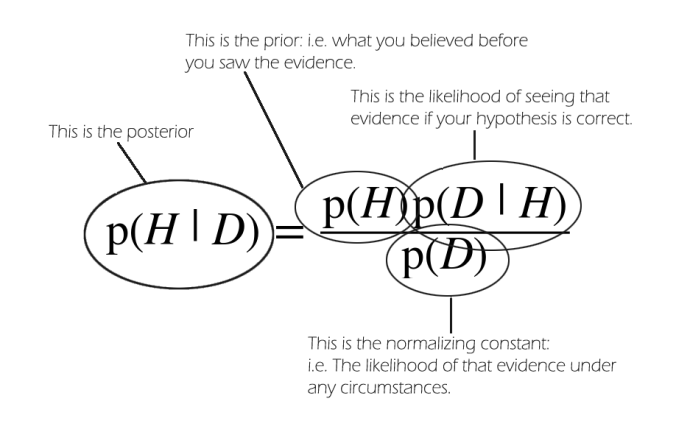
So we have an update rule of:
P(distance=40m | measured_rssi=-80) = P(measured_rssi = -80|distance=40m) * P(distance=40m)
Where we initially say that all distances within an area are equally likely = P(distance=40m) = 1/area
And we renormalize the probability to ensure that sum of probabilities over all distances = 1.
