I put together a ‘lie detector’ testing for galvanic skin response.
I didn’t work. I tested various obvious different ideas, such as looking at variances from a sliding window mean etc, but didn’t get anywhere.
It does light up if I hyperventilate though, which is er, useful? It is also, interestingly, lights up when my daughter uses it and shouts out swear words, which she finds highly amusing. I think it’s just detecting her jerking her hand around though. She doesn’t exactly sit still.
I used an op-amp to magnify the signal 200 times analogue-y (er, as opposed to digitally..), but I now wonder if I could use a high resolution (e.g. 40bit) digital to analog converter directly, and do more processing in software.
Perhaps even use a neural network to train to train it to detect lies.
I did order a 40bit AD evaluation board from TI, but haven’t had the chance to actually use it yet.
A friend told me of a non-deterministic bug that he had found that only crashed occasionally. He wrote a test case, ran it once, and the bug appeared after 3.5 hours of testing. He sent the bug report and test case to code owners, who ran it for 4 hours but couldn’t reproduce the bug. Intuitively we can see that they might have just been unlucky and thus not seen the crash.
So it got me wondering what the minimum amount of time that they need to run the test for, all other factors being equal, to be 95% likely to reproduce the bug again. (i.e. 2 sigma)
Assuming that the bug appears randomly, with an equal probability of per hour, then after 3.5 hours of running, there’s a probability of the bug appearing of:
Rearranging:
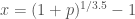
To have the tester reproduce the results in the end with a 95% chance, we need to 90% confidence in the probability of us producing the bug in the first place, and a 90% confidence of the reproducer reproducing the bug, so that combined we get a confidence in overall result. So the percentage chance, , of the observed outcome of seeing the crash after 3.5 hours is between 10% to 90%. Setting p to 0.1 and 0.9 in the above equation, we get that the probability of the bug appearing per hour is between 2.8% to 20%.
Taking the lowest probability, to get a total of 95% chance of reproducing the bug (and thus 90% chance of reproducing the bug GIVEN the probability of the bug appearing for us being 90%) we need to run for:
23 hours.
So to be 95% confident that the bug does not appear on the reproducer’s system, they would need to run the test case for 23 hours, assuming similar hardware etc.
This can be drastically brought down if the initial tester does a second run, to increase the value for .
Rerunning the test
The original tester reran the test himself and reproduced the bug 4 times and found that it always appeared in less than 6 hours.
To be 95% confidence in the overall results, and thus 90% confidence for just , we want the probability of the occurring 4 times in 4 runs in less than 6 hours to be 10%. Thus the probability of it occurring in 1 run in less than 6 hours is simply:
So setting p = 34% and using the equation above but with the number of hours set to 6, we get:
Which gives x = 5.0%. This means that with 90% confidence, the bug appears with a minimum probability of 5% per hour. So the amount of time, y, that the reproducer needs to run to be 95% likely to reproduce the bug is:
I wanted to do a physics-based layout in QML, to have bouncing bubbles etc.
D3.js has everything that I needed, but it needed to be tweaked to get it to run:
Create some dummy functions to stub the webbrowser javascript functions clearTimeout() and setTimeout() that we don’t have
Create a QML Timer to replace them and manually call force.tick()
Use dummy objects for D3 to manipulate, and then set the position of our real graphics to the determined position of the dummy objects. This is needed because D3 takes x,y coordinates to be the center of the object, whereas qml uses x,y to mean the top left.
It worked pretty well, and now I can do things like this in QML:
diff --git a/d3.js b/d3.js
index 8868e42..7aac164 100644
--- a/d3.js
+++ b/d3.js
@@ -1,4 +1,9 @@
-!function() {
-  var d3 = {
+function clearTimeout() {
+};
+function setTimeout() {
+};
+var d3;
+!function(){
+  d3 = {
     version: "3.5.5"
   };
@@ -9503,2 +9508,1 @@
-  this.d3 = d3;
-}();
\ No newline at end of file
+}();
(The ds.min.js file is also patched in the same way)
And in QML:
import QtQuick 2.2
import "."
import QtSensors 5.0
import "d3.js" as D3

Rectangle {
    id: bubbleContainer
    width: 1000
    height: 1000
    //clip: true

    property int numbubbles: 200;
    property real bubbleScaleFactor: 0.1
    property real maxBubbleRadius: width*0.15*bubbleScaleFactor + width/20*bubbleScaleFactor
    property variant bubblesprites: []

    function createBubbles() {
        var bubblecomponent = Qt.createComponent("bubble.qml");
        var radius = Math.random()*width*0.15*bubbleScaleFactor + width/20*bubbleScaleFactor
        bubblesprites.push(bubblecomponent.createObject(bubbleContainer, {"x": width/2-radius , "y": height/2 - radius, "radius":radius, "color":  "#ec7e78" } ));
        var xLeft = -radius
        var xRight = radius
        for (var i=1; i < numbubbles; ++i) {             var radius2 = Math.random()*width*0.15*bubbleScaleFactor + width/20*bubbleScaleFactor             var y = height*(0.5 + (Math.random()-0.5))-radius2             if (i % 2 === 0) {                 bubblesprites.push(bubblecomponent.createObject(bubbleContainer, {"x": xLeft, "y": y, "radius":radius2 } ));                 xLeft += radius2*2             } else {                 xRight -= radius2*2                 bubblesprites.push(bubblecomponent.createObject(bubbleContainer, {"x": xRight, "y": y, "radius":radius2 } ));             }         }     }     function boundParticle(b) {         if (b.y > height - b.radius)
            b.y = height - b.radius
        if (b.y < b.radius)             b.y = b.radius         if (b.x > width*2.5)
            b.x = width*2.5
        if (b.x < -width*2)
            b.x = -width*2
    }

    property real padding: width/100*bubbleScaleFactor;
    function collide(node) {
        var r = node.radius + maxBubbleRadius+10,
              nx1 = node.x - r,
              nx2 = node.x + r,
              ny1 = node.y - r,
              ny2 = node.y + r;
        boundParticle(node)
        return function(quad, x1, y1, x2, y2) {
            if (quad.point && (quad.point !== node)) {
              var x = node.x - quad.point.x,
                  y = node.y - quad.point.y,
                  l = Math.sqrt(x * x + y * y),
                  r = node.radius + quad.point.radius + padding;
              if (l < r) {                 l = (l - r) / l * .5;                 node.x -= x *= l;                 node.y -= y *= l;                 quad.point.x += x;                 quad.point.y += y;               }             }             return x1 > nx2 || x2 < nx1 || y1 > ny2 || y2 < ny1;
        };
    }

    property var nodes;
    property var force;

    Component.onCompleted: {
        initializeTimer.start()
    }

    Timer {
        id: initializeTimer
        interval: 20;
        running: false;
        repeat: false;
        onTriggered: {
            createBubbles();
            nodes = D3.d3.range(numbubbles).map(function() { return {radius: bubblesprites[this.index]}; });
            for(var i = 0; i < numbubbles; ++i) {
                nodes[i].radius = bubblesprites[i].radius;
                nodes[i].px = nodes[i].x = bubblesprites[i].x+bubblesprites[i].radius
                nodes[i].py = nodes[i].y = bubblesprites[i].y+bubblesprites[i].radius
            }
            nodes[0].fixed = true;

            force = D3.d3.layout.force().gravity(0.05).charge(function(d, i) { return 0; }).nodes(nodes).size([width,height])
            force.start()
            nodes[0].px = width/2
            nodes[0].py = height/2
            force.on("tick", function(e) {
                var q = D3.d3.geom.quadtree(nodes),i = 0,
                        n = nodes.length;
                while (++i < n) q.visit(collide(nodes[i]));
                for(var i = 0; i < numbubbles; ++i) {
                    bubblesprites[i].x = nodes[i].x - nodes[i].radius;
                    bubblesprites[i].y = nodes[i].y - nodes[i].radius;
                }
            });
            timer.start();
        }
    }

    Timer {
        id: timer
        interval: 26;
        running: false;
        repeat: true;
        onTriggered: {
            force.resume();
            force.tick();
        }
    }
}
I bought a 128×128 SPI Nokia 5110 display (The ILI9163) to hook up to an Arduino. I used an Arduino Mini which runs at 3.3v, since the display uses 3.3v logic.
Then wired it up like:
- LED       -->     +3.3V  -  (5V would work too)
- SCK       -->     Pin 13 -  Sclk,  (3.3V level)
- SDA       -->     Pin 11 -  Mosi,  (3.3V level)
- A0        -->     Pin 10 -  DC or RS pin (3.3V level)
- RST       -->     Pin 9  -  Or just connect to +3.3V
- CS        -->     Pin 8  -  CS pin (3.3V level)
- Gnd       -->     Gnd
- Vcc       -->     +3.3V
(Note that SDA and SCK pins aren’t optional, because we’re using the arduino SPI hardware to drive this. The DC and CS pins are changeable if you change the code)
And found a library to use this:
cd /libraries/
git clone https://github.com/adafruit/Adafruit-GFX-Library
git clone https://github.com/sumotoy/TFT_ILI9163C
I had to then edit TFT_ILI9163C/TFT_ILI9163C.h to comment out the #define __144_RED_PCB__ , and uncomment the #define __144_BLACK_PCB__ since my PCB was black. Without this change I got corruption on the top 1/4 of the screen.
Now to get something up and running, using the above pin definition:
This now gives us a black sceen with a yellow line. Woohoo!
Now, I have a bunch of images that I got an artist to draw, that look like:
I have 10 of these, and their raw size would be 128 * 128 * 4 * 10 = 655KB. Far too large for our 30KB of available flash memory on the nano!
But given the simplicity of the images, we can use a primitive compression algorithm and instead store these as Run Length Encoded. E.g. store as them as pixel index color followed by the number of pixels of that color in a line. We turn to trusty python to do this:
import os,sys
import itertools
from PIL import Image

rleBytes = 0
colorbits = 3

if len(sys.argv) != 3:
    print sys.argv[0], " <input file.png> <output file.h>"
    sys.exit()

def writeHeader(f):
    f.write("/* A generated file for a run length encoded image of " + sys.argv[1] + " */\n\n")
    f.write("#ifndef PIXEL_VALUE_TO_COLOR_INDEX\n")
    f.write("#define PIXEL_VALUE_TO_COLOR_INDEX(x) ((x) >> " + str(8-colorbits) + ")\n")
    f.write("#define PIXEL_VALUE_TO_RUN_LENGTH(x) ((x) & 0b" + ("1" *(8-colorbits)) + ")\n")
    f.write("#endif\n\n")
    f.write("namespace " + os.path.splitext(sys.argv[2])[0] + " {\n")
def writeFooter(f):
    f.write("}")

def writePalette(f, image):
    palette = image.im.getpalette()
    palette = map(ord, palette[:3*2**colorbits]) # This is now an array of bytes of the rgb565 values of the palette
    f.write("/* The RGB565 value for color 0 is in palette[0] and so on */\n")
    # convert from RGB888 to RGB565
    palette565 = [((palette[x] * 2**5 / 256) << 11) + ((palette[x+1] * 2**6 / 256) << 5) + ((palette[x+2] * 2**5/256)) for x in xrange(0, len(palette), 3)]
    f.write("const uint16_t palette[] PROGMEM = {" + ','.join(hex(x) for x in palette565) + "};\n\n")

def writePixel(pixelIndexColor, count):
    global rleBytes
    f.write(hex((pixelIndexColor << (8 - colorbits)) + count) + "," )
    rleBytes += 1

def writePixels(f):
    f.write("/* The first (MSB) " + str(colorbits) + "bits of each byte represent the color index, and the last " + str(8-colorbits) + " bits represent the number of pixels of that color */\n")
    f.write("const unsigned char pixels[] PROGMEM = {")
    (width, height) = image.size

    lastColors = []
    lastColor = -1
    lastColorCount = 0
    for y in xrange(height):
        for x in xrange(width):
            color = pix[x,y]
            if lastColorCount +1 < 2**(8 - colorbits) and (lastColorCount == 0 or color == lastColor):
                lastColorCount = lastColorCount + 1
            else:
                writePixel(lastColor, lastColorCount)
                lastColorCount = 1
            lastColor = color
        # To make the decoder easier, truncate at the end of a row
        # This adds about 5% to the total file size though
        writePixel(lastColor, lastColorCount)
        lastColorCount = 0
    f.write("};\n\n");


image = Image.open(sys.argv[1])
image = image.convert("P", palette=Image.ADAPTIVE, colors=2**colorbits)
#image.save("tmp.png")
pix = image.load()

f = open(sys.argv[2], 'w')
writeHeader(f)
writePalette(f, image)
writePixels(f)
writeFooter(f)
f.close()

print "Summary: Total Bytes: ", rleBytes
The result is that the 10 pictures take up 14kb. This doesn’t produce an optimal image, but it’s a decent starting point. This generates header files like:
/* A generated file for a run length encoded image of face1.png */

#ifndef PIXEL_VALUE_TO_COLOR_INDEX
#define PIXEL_VALUE_TO_COLOR_INDEX(x) ((x) >> 5)
#define PIXEL_VALUE_TO_RUN_LENGTH(x) ((x) & 0b11111)
#endif

namespace face1 {
/* The RGB565 value for color 0 is in palette[0] and so on */
const uint16_t palette[] PROGMEM = {0xef0b,0xf4a3,0x0,0xdb63,0xffff,0xa302,0xe54a,0x5181};

/* The first (MSB) 3 bits of each byte represent the color index, and the last 5 bits represent the number of pixels of that color */
const unsigned char pixels[] PROGMEM = {0x5f,0x56,0xe2...}
}
Which represents the image:
Which isn’t too bad for a first go. (This was generated by adding a image.save('tmp.png')" in the python code after converting the image).
Now we need an arduino sketch to pull this all in:
#include <SPI.h>
#include <Adafruit_GFX.h>
#include <TFT_ILI9163C.h>
#include "face1.h"
#include "face2.h"
#include "face3.h"
#include "face4.h"
#include "face5.h"
#include "face6.h"
#include "face7.h"
#include "face8.h"
#include "face9.h"
#include "face10.h"

const unsigned char *pixels[] = { face1::pixels, face2::pixels, face3::pixels, face4::pixels, face5::pixels, face6::pixels, face7::pixels, face8::pixels, face9::pixels, face10::pixels } ;
const unsigned char numpixels[] = { sizeof(face1::pixels), sizeof(face2::pixels), sizeof(face3::pixels), sizeof(face4::pixels), sizeof(face5::pixels), sizeof(face6::pixels), sizeof(face7::pixels), sizeof(face8::pixels), sizeof(face9::pixels), sizeof(face10::pixels) };
const uint16_t *palette[] = { face1::palette, face2::palette, face3::palette, face4::palette, face5::palette, face6::palette, face7::palette, face8::palette, face9::palette, face10::palette } ;


/*
 We are using 4 wire SPI here, so:
 MOSI:  11
 SCK:   13
 the rest of pin below:
 */
#define __CS 8
#define __DC 10
#define __RESET 9
TFT_ILI9163C tft = TFT_ILI9163C(__CS, __DC, __RESET);

const uint16_t width = 128;
const uint16_t height = 128;

void drawFace(int i);

void setup(void) {
  tft.begin();
}


void drawImage(const unsigned char *pixels, const unsigned char numPixels, const uint16_t *palette) {
  int16_t x = 0;
  int16_t y = 0;
  for( int i = 0; i < sizeof(face1::pixels); ++i) {
    unsigned char pixel = pgm_read_byte_near(pixels + i);
    /* The first (MSB) 3 of each byte represent the color index, and the last 5 bits represent the number of pixels of that color */
    unsigned char colorIndex = PIXEL_VALUE_TO_COLOR_INDEX(pixel);
    int16_t count = PIXEL_VALUE_TO_RUN_LENGTH(pixel);
    uint16_t color = pgm_read_word_near(palette + colorIndex);
    tft.drawFastHLine(x,y,count+1,color);
    x += count;
    if(x >= width) {
      x = 0;
      y+=1;
    }
  }
}

void loop() {
  for(int i = 1; i <= 10; ++i)
    drawFace(i);
}

void drawFace(int i) {
  drawImage(pixels[i-1], numpixels[i-1], palette[i-1]);
}
Pretty straight forward.
Using 4 bits per color uses up slightly too much space: 34,104 bytes (111%) of program storage.
Using 3 bits per color introduces slight artifcats, but presumably removable if we tweak the images, but it fits with plenty of room to space:
Sketch uses 20,796 bytes (67%) of program storage space. Maximum is 30,720 bytes.
Global variables use 134 bytes (6%) of dynamic memory, leaving 1,914 bytes for local variables. Maximum is 2,048 bytes.
The result is this:
Note that this is actually updating at maximum speed. There is room for improvement in the adafruit graphics code however, so I may have a go at improving this if I need faster updates. It might be nice to faster updates anyway in order to minimize battery use.
Android Phone App
I wanted to keep the Android app side of it as clean and simple as possible. There’s not much to document regarding the GUI side of things – it’s a pretty straightforward Android app.
The idea here is to connect via bluetooth to both the arduino and to a Healthband. It measures the heart rate and, more importantly, the very slightly changes in time between the heart pulses. By the knowing the users age, sex and weight, we can calculate the amount of stress that they are currently experiencing. We can then display that in the app, and send that information via Bluetooth Low Energy to our arduino heart badge.
It perhaps needs some tweaking – I’m not really that angry, honest! Lots of polishing is still needed, but the barebones are starting to come together!
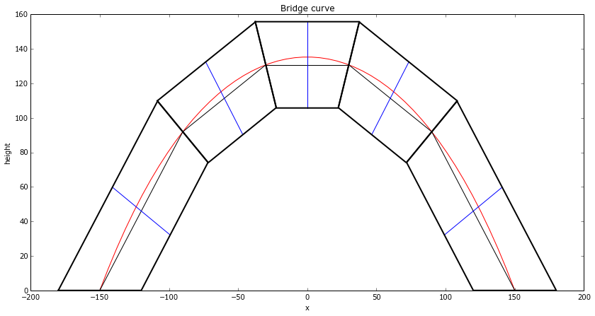
Now we have to decide how to cut the wood. To produce the arch, the angle of each piece of wood (the tangent lines), relative to the horizontal, is just: . So the angle between two adjacent pieces of wood is the difference between their angles.
The wood will be parallel with those tangent lines, so we can draw on the normal lines for those tangent lines, of the thickness of the wood:
def dy(x):
    '''return an approximation of dy/dx'''
    return (y(x+0.05) - y(x-0.05)) / 0.1

def normalAngle(x):
    if x == -L/2:
        return 0
    elif x == L/2:
        return math.pi
    return math.atan2(-1.0, dy(x));

WoodThickness = 50.0 # in millimeters

def getNormalCoords(x, ymidpoint, lineLength):
    tangent = dy(x)
    if tangent != 0:
        if x == -L/2 or x == L/2:
            normalSlope = 0
        else:
            normalSlope = -1 / dy(x)
        xlength = lineLength * math.cos(normalAngle(x))
        xstart = x-xlength/2
        xend = x+xlength/2
        ystart = ymidpoint + normalSlope * (xstart - x)
        yend = ymidpoint + normalSlope * (xend - x)
    else:
        xstart = x
        xend = x
        ystart = ymidpoint + lineLength/2
        yend = ymidpoint - lineLength/2
    return (xstart, ystart, xend, yend)

for block in blocks:
    (xstart, ystart, xend, yend) = getNormalCoords(block.midpoint_x, block.midpoint_y, WoodThickness)
    ax.plot([xstart, xend], [ystart, yend], 'b-', lw=1)
fig
Now, the red curve is going to represent the line of force. My reasoning is that if there was any force normal to the red curve, then the string/bridge/weight would thus accelerate and change position.
So to minimize the lateral forces where the wood meets, we want the wood cuts to be normal to the red line. We add that, then draw the whole block:
def getWoodCorners(block, x):
    ''' Return the top and bottom of the piece of wood whose cut passes through x,y(x), and whose middle is at xmid '''
    adjusted_thickness = WoodThickness / math.cos(normalAngle(x) - normalAngle(block.midpoint_x))
    return getNormalCoords(x, y(x), adjusted_thickness)

def drawPolygon(coords, linewidth):
    xcoords,ycoords = zip(*coords)
    xcoords = xcoords + (xcoords[0],)
    ycoords = ycoords + (ycoords[0],)
    ax.plot(xcoords, ycoords, 'k-', lw=linewidth)

#Draw all the blocks
for block in blocks:
    (xstart0, ystart0, xend0, yend0) = getWoodCorners(block, block.start_x) # Left side of block
    (xstart1, ystart1, xend1, yend1) = getWoodCorners(block, block.end_x) # Right side of block
    block.coords = [ (xstart0, ystart0), (xstart1, ystart1), (xend1, yend1), (xend0, yend0) ]
    drawPolygon(block.coords, 2) # Draw block

fig
There’s a few things to note here:
The code appears to do some pretty redundant calculations when calculating the angles – but much of this is to make the signs of the angles correct. It’s easier and nicer to let atan2 handle the signs for the quadrants, than to try to simplify the code and handle this ourselves.
The blocks aren’t actually exactly the same size at the points where they meet. The differences are on the order of 1%, and not noticeable in these drawings however.
Now we need to draw and label these blocks in a way that makes it easiest to cut:
fig, ax = subplots(1,1)
fig.set_size_inches(17,7)
axis('off')

def rotatePolygon(polygon,theta):
    """Rotates the given polygon which consists of corners represented as (x,y), around the ORIGIN, clock-wise, theta radians"""
    return [(x*math.cos(theta)-y*math.sin(theta) , x*math.sin(theta)+y*math.cos(theta)) for (x,y) in polygon]

def translatePolygon(polygon, xshift,yshift):
    """Shifts the polygon by the given amount"""
    return [ (x+xshift, y+yshift) for (x,y) in polygon]

sawThickness = 3.0 # add 3 mm gap between blocks for saw thickess
#Draw all the blocks
xshift = 10.0 # Start at 10mm to make it easier to cut by hand
topCutCoords = []
bottomCutCoords = []
for block in blocks:
    coords = translatePolygon(block.coords, -block.midpoint_x, -block.midpoint_y)
    coords = rotatePolygon(coords, -block.angle())
    coords = translatePolygon(coords, xshift - coords[0][0], -coords[3][1])
    xshift = coords[1][0] + sawThickness
    drawPolygon(coords,1)
    (topLeft, topRight, bottomRight, bottomLeft) = coords
    itopLeft = int(round(topLeft[0]))
    itopRight = int(round(topRight[0]))
    ibottomLeft = int(round(bottomLeft[0]))
    ibottomRight = int(round(bottomRight[0]))
    topCutCoords.append(itopLeft)
    topCutCoords.append(itopRight)
    bottomCutCoords.append(ibottomLeft)
    bottomCutCoords.append(ibottomRight)
    ax.text(topLeft[0], topLeft[1], itopLeft)
    ax.text(topRight[0], topRight[1], itopRight, horizontalalignment='right')
    ax.text(bottomLeft[0], bottomLeft[1], ibottomLeft, verticalalignment='top', horizontalalignment='center')
    ax.text(bottomRight[0], bottomRight[1], ibottomRight, verticalalignment='top', horizontalalignment='center')

print "Top coordinates:", topCutCoords
print "Bottom Coordinates:", bottomCutCoords
I wanted to have a modern aerodynamics simulator, to test out my flight control hardware and software.
Apologies in advance for a very terse post. I spent a lot of hours in a very short timespan to do this as a quick experiment.
So I used Unreal Engine 4 for the graphics engine, and built on top of that.
The main forces for a low speed aircraft that I want to model:
The lift force due to the wing
The drag force due to the wind
Gravity
Any horizontal forces from propellers in aircraft-style propulsion
Any vertical forces from propellers in quadcopter-style propulsion
Lift force due to the wing
The equation for the lift force is:
I created a function for the lift coefficient, , based on the angle, by calculating it theoretically. To get proper results, I would need to actually measure this in a wind tunnel, but this is good enough for a first approximation:
The horizontal axis is the angle of attack, in degrees. When the aircraft is flying “straight”, the angle of attack is not usually 0, but around 5 to 10 degrees, thus still providing an upward force.
I repeat this for each force in turn.
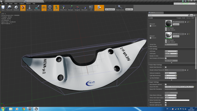
3D Model
To visualize it nicely, I modelled the craft in blender, manually set the texture space, and painted the texture in gimp. As you can tell from the texture space, there are several horrible problems with the geometry ‘loops’. But it took a whole day to get the top and bottom looking decent, and it was close enough for my purposes.
I imported the model into Unreal Engine 4, and used a high-resolution render for the version in the top right, and used a low-resolution version for the game.
Next, here’s the underneath view. You can see jagged edges in the model here, because at the time I didn’t understand how normal smoothing worked. After a quick google, I selected those vertexes in blender and enabled normal smoothing on them and fixed that.
and then finally, testing it out on the real thing:
Architecture
The architecture is a fairly standard Hardware-in-loop system.
The key modules are:
The Flight Controller which controls the craft. This is not used if we are connected to external real hardware, such as the my controller.
The Communication Module to the real hardware, receiving information about the desired thrust of the engines and the Radio Control inputs from the user, and sending information about the current simulated position and speed.
The Physics Simulator which calculates the physical forces on the craft and applies them.
The User Interface which displays a lot of information about the craft as well as the internal controller.
The low level flight controller and network communication code is written in C++. Much of the high level logic is written in a visual language called ‘Blueprint’.
User Interface
From the GUI User Interface, you can control:
The aerodynamic forces on the wings
The height above ground to air pressure curve
The wing span and aerofoil chord length
The moment of inertia
The thrust of the turbines
The placement of the turbines
The PID values for the internal controller
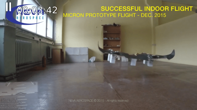
Result
It worked pretty well.
It uses Hardware-In-Loop to allow the real hardware to control this, including a RC-Transmitter.
In this video I am allowing the PID algorithms to control the roll, pitch, yaw and height, which I then add to in order to control it.
PID Tuning
I implemented an auto-tuner for the PID algorithm, which you can tune and trigger from the GUI.
Hardware
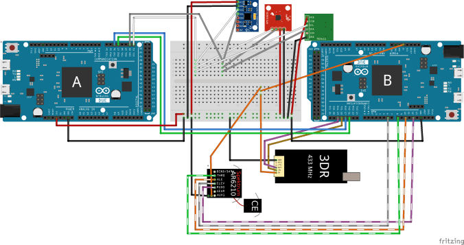
I used two arduinos to control the system:
And set up the Arduinos as so: (Btw, I used the Fritzing software for this – it’s pretty cool).
And putting together the hardware for testing (sorry for the mess). (I’m using QGroundControl to test it out).
And then mounting the hardware on a bit of wood as a base to keep it all together and make it more tidy:
I will hopefully later make a post about the software controlling this.
ESC Motor Controller Delay
I was particularly worried about the delay that the controller introduces.
I modified the program and used a basic UFO style quadcopter, then added in a 50ms buffer, to test the reaction.
For reference, here’s a photo of the real thing that I work on:
The quadcopter is programmed to try to hover over the chair.
I also tested with different latencies:
50ms really is the bare minimum that you can get away with.
These are manually tuned PIDs.
I did also simulate this system in 1D in Matlab’s Simulink:
A graph of the amplitude:
And finally, various bode plots etc. Just click on any for a larger image. Again, apologies for the awful terseness.
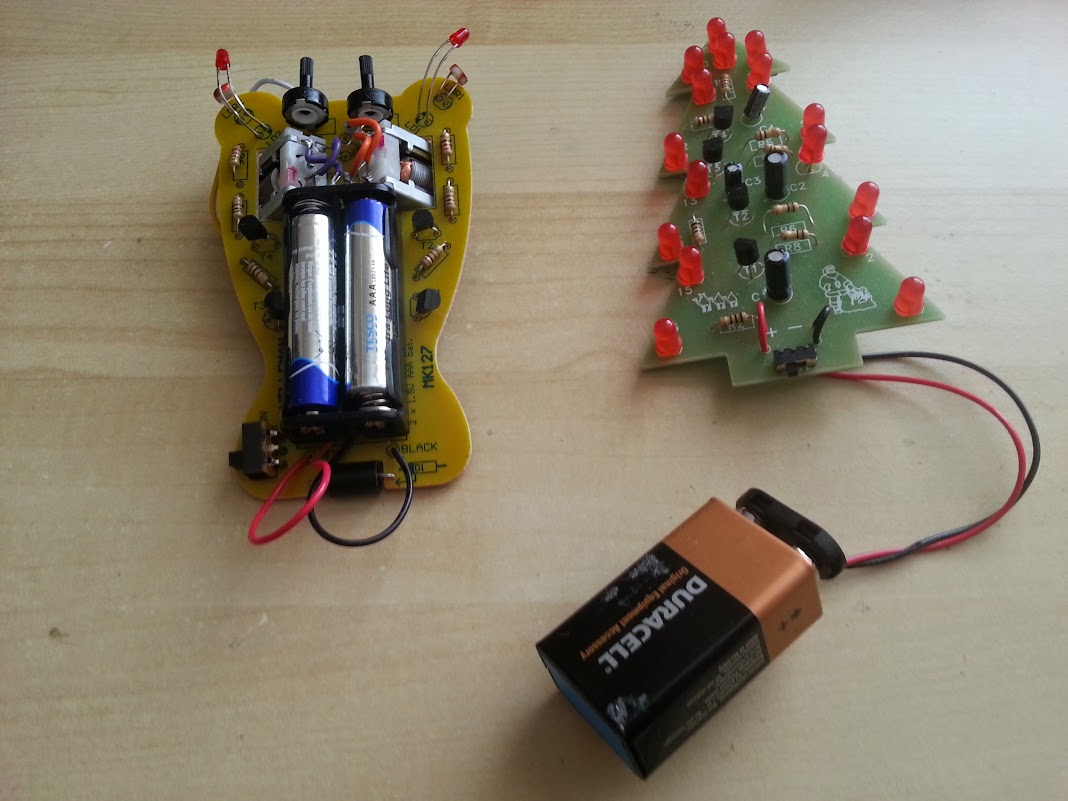
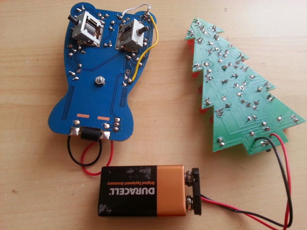
I’ve been trying to introduce my daughter, 6 years old, to electronics. I started her on the Velleman MK100 Electronic Christmas Tree which went fairly smoothly.
The problem with these kits is that beginners will make mistakes that will be unable to recover from. Not only that, but they don’t explain how they work so you can’t debug them or understand what you are doing.
On top of that, the bots can be outright hackish – for example, requiring you to scrap the edge of the motors, and then solder the chasis of the motor directly to the board at an angle! And this is even more difficult than it sounds, since the motor is highly magnetic and so requires a steady strong hand to keep the soldering iron still.
This was the result:
Notice the four wires from the motor. This was because we put the motors in the wrong way around, despite following the instructions. So I had to reverse the motors. This sort of repair is probably beyond a child. But worse:
Notice the yellow and white wires? This is another repair job after finding that the light sensitive resistor had broken the bottom of the board and was not making a proper connection. Pretty much impossible to detect this for a novice or if you didn’t have a voltmeter.
I’m not sure what the solution is. In the past I’ve used various non-soldering electronics kits, but they all have their own disadvantages.
I previously talked about the code for the display driver, and the code for the snake AI algorithm, but here I want to just tie it all together.
I used the arduino tools, setup like so:
I initially made a mistake and used the default 5V option with the 3V board. It uploaded correctly, but the serial output was at half the expected speed. This is because the 5V board runs at 16mhz, but the 3.3V board runs at 8Mhz. (As a side note, I searched for the particle AVR chip and it’s actually rated at 20mhz and 10mhz respectively. I wonder why the Arduino underclocks the processor? As a second side note, for fun I tested a 5V board at 16mhz but actually fed it 3.3V and amazingly it worked. Obviously reliability is probably an issue, but the tolerance for low voltage is well outside the official specs, so in pinch you can really abuse this hardware. I got it down to 3.1V before the 5V board gave up).
Programming for the PC
I wrote the code such that the arduino-specific code was as minimal as possible, and kept in .ino files. And the rest of the code in .cpp files. The result was that I could do almost all the development and debugging for the PC.
Although this was slightly more work (e.g. I had to write an ncurses output), it was very much worth it. I compiled the program with:
The sanitize=address option is new to GCC 4.8.0 and is extremely cool. It’s a memory error checker and it saved my bacon several times. For me, it has replaced valgrind’s memchecker tool.
Monitoring memory usage
I needed to be aware of every byte of memory that I used throughout the project, and to compare my theoretical counting against actual usage I used a pretty neat trick that I found on the internet:
  static int freeRam ()
  {
    extern int __heap_start, *__brkval;
    int v;
    return (int) &v - (__brkval == 0 ? (int) &__heap_start : (int) __brkval);
  }
This function returns the amount of free memory by taking the current stack position (since v is on the stack), and taking the difference to the current heap position. This works because on arduino the heap and stack grow towards each other, like this:
Final product
Final product uses 1.4KB out of the 2KB of memory available.
We need an AI that can play a perfect game of Snake. To collect the food without crashing into itself.
But it needs to run in real time on an 8Mhz processor, and use around 1 KB of memory. The extreme memory and speed restrictions means that we do not want to allocate any heap memory, and should run everything on the stack.
None of the conventional path finding algorithms would work here, so we need a new approach. The trick here is to realise that in the end part of the game, the snake will be following a planar Hamiltonian Cycle of a 2D array:
So what we can do is precompute a random hamiltonian cycle at the start of each game, then have the snake follow that cycle. It will thus pass through every point, without risk of crashing, and eventually win the game.
There are various way to create a hamiltonian cycle, but one way is to use Prim’s Algorithm to generate a maze of half the width and half the height. Then walk the maze by always turning left when possible. The resulting path will be twice the width and height and will be a hamiltonian cycle.
Now, we could have the snake just follow the cycle the entire time, but the result is very boring to watch because the snake does not follow the food, but instead just follows the preset path.
To solve this, I invented a new algorithm which I call the pertubated hamiltonian cycle. First, we imagine the cycle as being a 1D path. On this path we have the tail, the body, the head, and (wrapping back round again) the tail again.
The key is realising that as long as we always enforce this order, we won’t crash. As long as all parts of the body are between tail and the head, and as long as our snake does not grow long enough for the head to catch up with the tail, we will not crash.
This insight drastically simplifies the snake AI, because now we only need to worry about the position of the head and the tail, and we can trivially compute (in O(1)) the distance between the head and tail since that’s just the difference in position in the linear 1D array:
Now, this 1D array is actually embedded in a 2D array, and the head can actually move in any of 3 directions at any time. This is equivalent to taking shortcuts through the 1D array. If we want to stick to our conditions, then any shortcut must result in the head not overtaking the tail, and it shouldn’t overtake the food, if it hasn’t already. We must also leave sufficient room between the head and tail for the amount that we expect to grow.
Now we can use a standard shortest-path finding algorithm to find the optimal shortcut to the food. For example, an A* shortest path algorithm.
However I opted for the very simplest algorithm of just using a greedy search. It doesn’t produce an optimal path, but visually it was sufficiently good. I additionally disable the shortcuts when the snake takes up 50% of the board.
To test, I started with a simple non-random zig-zag cycle, but with shortcuts:
What you can see here is the snake following the zig-zag cycle, but occasionally taking shortcuts.
We can now switch to a random maze:
And once it’s working on the PC, get it working on the phone:
Code
NOTE: I have lost the original code, but I’ve recreated it and put it here:
First, the pin mappings as shown in the previous diagram:
                     // Description  Pin on LCD display
                     // LCD Vcc .... Pin 1 +3.3V (up to 7.4 mA) Chip power supply
#define PIN_SCLK  2  // LCD SPIClk . Pin 2 Serial clock line of LCD                          // Was 2 on 1st prototype
#define PIN_SDIN  5  // LCD SPIDat . Pin 3 Serial data input of LCD                          // Was 5 on 1st prototype
#define PIN_DC    3  // LCD Dat/Com. Pin 4 (or sometimes labelled A0) command/data switch    // Was 3 on 1st prototype
                     // LCD CS  .... Pin 5 Active low chip select (connected to GND)
                     // LCD OSC .... Pin 6 External clock, connected to vdd
                     // LCD Gnd .... Pin 7 Ground for VDD
                     // LCD Vout ... Pin 8 Output of display-internal dc/dc converter - Left floating - NO WIRE FOR THIS.  If we added a wire, we could connect to gnd via a 100nF capacitor
#define PIN_RESET 4  // LCD RST .... Pin 9 Active low reset   // Was 4 on prototype
#define PIN_BACKLIGHT 6 // - Backlight controller. Optional.  It's connected to a transistor that should be connected to Vcc and gnd

#define LCD_C     LOW
#define LCD_D     HIGH
We need to initialize the LCD:
void LcdClear(void)
{
  for (int index = 0; index < LCD_X * LCD_Y / 8; index++)
    LcdWrite(LCD_D, 0x00);
}

void LcdInitialise(void)
{
 // pinMode(PIN_SCE, OUTPUT);
  pinMode(PIN_RESET, OUTPUT);
  pinMode(PIN_DC, OUTPUT);
  pinMode(PIN_SDIN, OUTPUT);
  pinMode(PIN_SCLK, OUTPUT);
  pinMode(PIN_BACKLIGHT, OUTPUT);
  digitalWrite(PIN_RESET, LOW); // This must be set to low within 30ms of start up, so don't put any long running code before this
  delay(30); //The res pulse needs to be a minimum of 100ns long, with no maximum.  So technically we don't need this delay since a digital write takes 1/8mhz = 125ns.  However I'm making it 30ms for no real reason
  digitalWrite(PIN_RESET, HIGH);
  digitalWrite(PIN_BACKLIGHT, HIGH);
  LcdWrite(LCD_C, 0x21 );  // LCD Extended Commands.
  LcdWrite(LCD_C, 0x80 + 0x31 ); // Set LCD Vop (Contrast).  //0x80 + V_op    The LCD voltage is:  V_lcd = 3.06 + V_op * 0.06
  LcdWrite(LCD_C, 0x04 + 0x0 );  // Set Temp coefficent. //0 = Upper Limit.  1 = Typical Curve.  2 = Temperature coefficient of IC.  3 = Lower limit
  LcdWrite(LCD_C, 0x10 + 0x3 );  // LCD bias mode 1:48. //0x10  + bias mode.  A bias mode of 3 gives a "recommended mux rate" of 1:48
  LcdWrite(LCD_C, 0x20 );  // LCD Basic Commands
  LcdWrite(LCD_C, 0x0C );  // LCD in normal mode.
}

/* Write a column of 8 pixels in one go */
void LcdWrite(byte dc, byte data)
{
  digitalWrite(PIN_DC, dc);
  shiftOut(PIN_SDIN, PIN_SCLK, MSBFIRST, data);
}

/* gotoXY routine to position cursor
   x - range: 0 to 84
   y - range: 0 to 5
*/
void gotoXY(int x, int y)
{
  LcdWrite( 0, 0x80 | x);  // Column.
  LcdWrite( 0, 0x40 | y);  // Row.
}
So this is pretty straightforward. We can’t write per pixel, but must write a column of 8 pixels at a time.
This causes a problem – we don’t have enough memory to make a framebuffer (we have only 2kb in total!), so all drawing must be calculated on the fly, with the whole column of 8 pixels calculated on the fly.
Snake game
The purpose of all of this is to create a game of snake. In our game, we want the snake to be 3 pixels wide, with a 1 pixel gap. It must be offset by 2 pixels though because of border.
The result is code like this:
/* x,y are in board coordinates where x is between 0 to 19 and y is between 0 and 10, inclusive*/
void update_square(const int x, const int y)
{
  /* Say x,y is board square 0,0  so we need to update columns 1,2,3,4
   * and rows 1,2,3,4  (column and row 0 is the border).
   * But we have actually update row 0,1,2,3,4,5,6,7  since that's how the
   * lcd display works.
   */
  int col_start = 4*x+1;
  int col_end = col_start+3; // Inclusive range
  for(int pixel_x = col_start; pixel_x <= col_end; ++pixel_x) {
    int pixelrow_y_start = y/2;
    int pixelrow_y_end = (y+1)/2; /* Inclusive.  We are updating either 1 or 2 lcd block, each with 2 squares */
    int current_y = pixelrow_y_start*2;
    for(int pixelrow_y = pixelrow_y_start; pixelrow_y <= pixelrow_y_end; ++pixelrow_y, current_y+=2) {
      /* pixel_x is between 0 and 83, and pixelrow_y is between 0 and 5 inclusive */
      int number = 0; /* The 8-bit pixels for this column */
      if(pixelrow_y == 0)
        number = 0b1; /* Top border */
      else
        number = get_image(x, current_y-1, (pixel_x-1)%4) >> 3;
      if( current_y < ARENA_HEIGHT) {
        number |= (get_image(x, current_y, (pixel_x-1)%4) << 1);
        number |= (get_image(x, current_y+1, (pixel_x-1) %4) << 5);
      }
      gotoXY(pixel_x, pixelrow_y);
      LcdWrite(1,number);
    }
  }
}

int get_image(int x, int y, int column)
{
  if( y >= ARENA_HEIGHT)
    return 0;
  int number = 0;
  if( y == ARENA_HEIGHT-1 )
    number = 0b0100000; /* Bottom border */

  if(board.hasSnake(x,y))
    return number | get_snake_image(x, y, column);

  if(food.x == x && food.y == y)
    return number | get_food_image(x, y, column);

  return number;
}

int get_food_image(int x, int y, int column)
{
  if(column == 0)
    return 0b0000;
  if(column == 1)
    return 0b0100;
  if(column == 2)
    return 0b1010;
  if(column == 3)
    return 0b0100;
}

/* Column 0 and row 0 is the gap between the snake*/

/* Column is 0-3 and this returns a number between
 * 0b0000 and 0b1111 for the pixels for this column
   The MSB (left most digit) is drawn below the LSB */
int get_snake_image(int x, int y, int column)
{
  if(column == 0) {
    if(board.snakeFromLeft(x,y))
      return 0b1110;
    else
      return 0;
  }
  if(board.snakeFromTop(x,y))
    return 0b1111;
  else
    return 0b1110;
}
Pretty messy code, but necessary to save every possible byte of memory.
Now we can call
update_square(x,y)
when something changes in board coordinates x,y, and this will redraw the screen at that position.
So now we just need to implement the snake logic to create a snake and get it to play automatically. And do so in around 1 kilobyte of memory!

 per hour, then after 3.5 hours of running, there’s a probability
  of the bug appearing of:

 confidence in overall result. So the percentage chance,
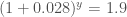

 23 hours.
 , we want the probability of the occurring 4 times in 4 runs in less than 6 hours to be 10%. Thus the probability of it occurring in 1 run in less than 6 hours is simply:
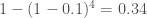


 . So the angle between two adjacent pieces of wood is the difference between their angles.


 , based on the angle, by calculating it theoretically. To get proper results, I would need to actually measure this in a wind tunnel, but this is good enough for a first approximation:
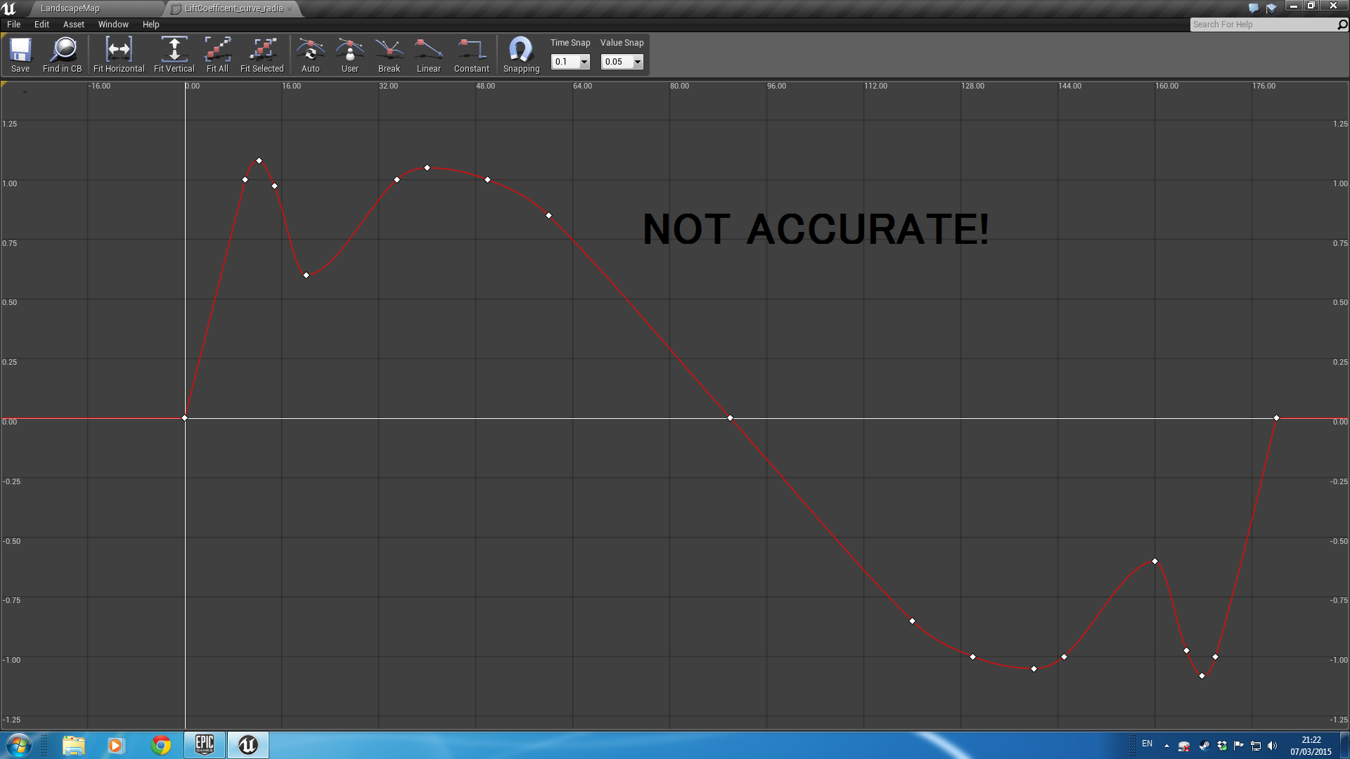


")