I wanted to bend a large amount of wire for another project.
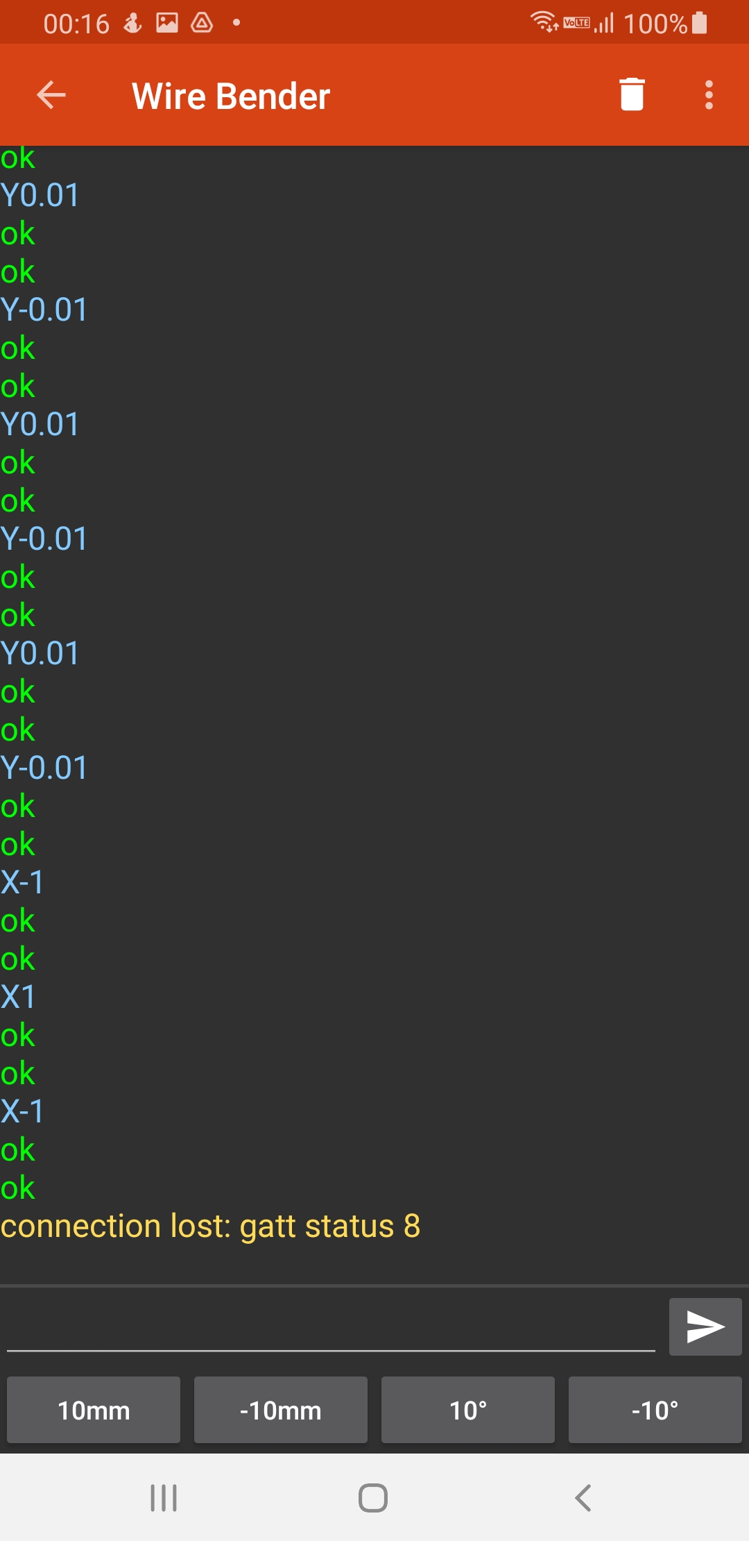
So I made this, a phone controlled wire bender. You plug it, establish a Bluetooth connection to it, and use the nifty android app I made to make it bend wire.

Details
I had an idea that an 3d printer’s extruder could also be used to extrude wire. So mocked something up:

And then laser cut it.
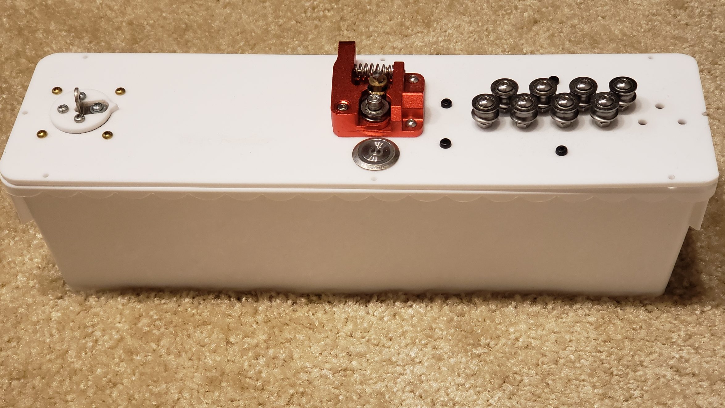
Mounting
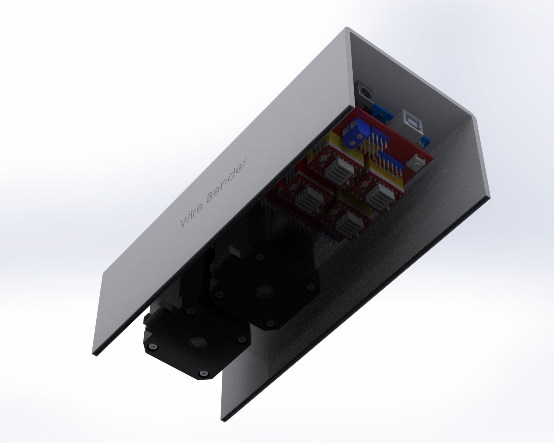
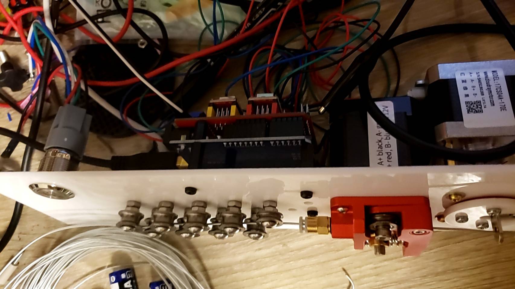
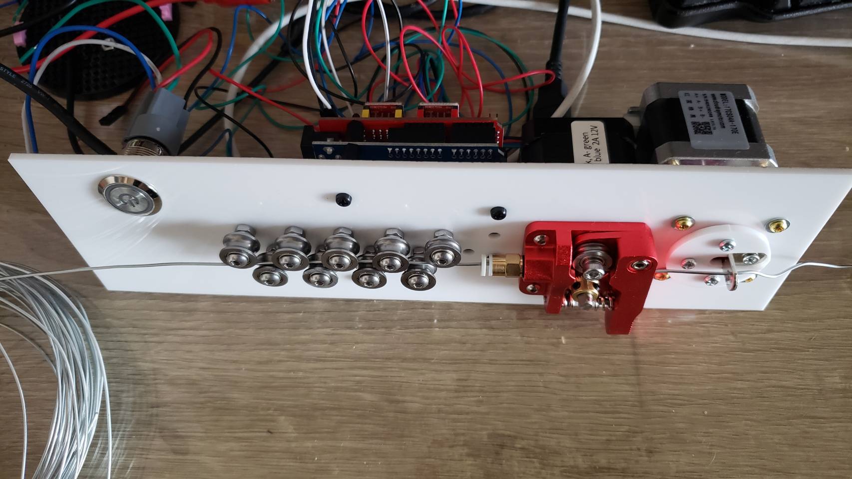
I decided to mount everything to top acrylic, except for the power connector.
Also, I didn’t do much wire management 🙂

The “project box” is actually a flower pot 🙂
One thing I didn’t foresee with mounting everything upside down is that one of the heatsinks on the motor controller fell off. I had to add an acrylic plate on top to hold them in place. Also, I think I need some active cooling. I haven’t had any actual problems yet, despite bending a lot of wire, but I’m sure I’m doing the controllers and motors no favors.
Previous iterations
I actually went through quite a few iterations. Here was one of the first designs, before I realized that I needed the wire bending part to be much further away from the extruder:


I went through a few different iterations. The set of 11 feeder ball-bearings are there to straighten the wire. It’s not obvious, but they actually converge at approximately a 2 degree angle, and I find this works best. So when the wire is initially fed in, the large spaced bearings smooth out the large kinks, and then the closer spaced bearings smooth out the small kinks. Try trying to do it all in one pass doesn’t work because the friction ends up being too high.
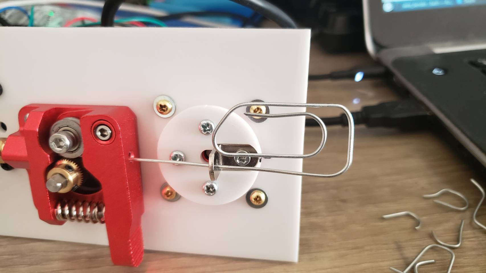
I replaced the extruder feeder with one with a much more ‘grippy’ surface. The grooved metal needs to be harder than the wire you’re feeding into it, so that it can grip it well. This did result in marks in the metal, but that was okay for my purpose. Using two feeder motors could help with this.

Algorithm
The algorithm to turn an arbitrary shape into a set of motor controls was actually pretty interesting, and a large part of the project. Because you have to bend the wire further than the angle you actually want, because it springs back. I plan to write this part up properly later.
Software control
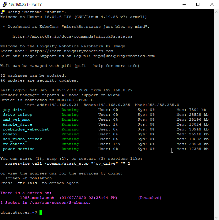
For computer control, I connect the stepper motors to a stepper motor driver, which I connect to an Arduino, which communicates over bluetooth serial to an android app. For prototyping I actually connected it to my laptop, and wrote a program in python to control it.


Both programs were pretty basic, but the android app has a lot more code for UI, bluetooth communication etc. The python code is lot easier to understand:
#!/usr/bin/env python3

import serial
import time
from termcolor import colored
from typing import Union
try:
    import gnureadline as readline
except ImportError:
    import readline

readline.parse_and_bind('tab: complete')
baud=9600 # We override Arduino/libraries/grbl/config.h to change to 9600
# because that's the default of the bluetooth module

try:
    s = serial.Serial('/dev/ttyUSB0',baud)
    print("Connected to /dev/ttyUSB0")
except:
    s = serial.Serial('/dev/ttyUSB1',baud)
    print("Connected to /dev/ttyUSB1")

# Wake up grbl
s.write(b"\r\n\r\n")
time.sleep(2)   # Wait for grbl to initialize
s.flushInput()  # Flush startup text in serial input

def readLineFromSerial():
    grbl_out: bytes = s.readline() # Wait for grbl response with carriage return
    print(colored(grbl_out.strip().decode('latin1'), 'green'))

def readAtLeastOneLineFromSerial():
    readLineFromSerial()
    while (s.inWaiting() > 0):
        readLineFromSerial()

def runCommand(cmd: Union[str, bytes]):
    if isinstance(cmd, str):
        cmd = cmd.encode('latin1')
    cmd = cmd.strip() # Strip all EOL characters for consistency
    print('>', cmd.decode('latin1'))
    s.write(cmd + b'\n') # Send g-code block to grbl
    readAtLeastOneLineFromSerial()

motor_angle: float = 0.0
MICROSTEPS: int = 16
YSCALE: float = 1000.0

def sign(x: float):
    return 1 if x >= 0 else -1

def motorYDeltaAngleToValue(delta_angle: float):
    return delta_angle / YSCALE

def motorXLengthToValue(delta_x: float):
    return delta_x

def rotateMotorY_noFeed(new_angle: float):
    global motor_angle
    delta_angle = new_angle - motor_angle
    runCommand(f"G1 Y{motorYDeltaAngleToValue(delta_angle):.3f}")
    motor_angle = new_angle

def rotateMotorY_feed(new_angle: float):
    global motor_angle
    delta_angle = new_angle - motor_angle
    motor_angle = new_angle
    Y = motorYDeltaAngleToValue(delta_angle)

    wire_bend_angle = 30 # fixme
    bend_radius = 3
    wire_length_needed = 3.1415 * bend_radius * bend_radius * wire_bend_angle / 360
    X = motorXLengthToValue(wire_length_needed)
    runCommand(f"G1 X{X:.3f} Y{Y:.3f}")

def rotateMotorY(new_angle: float):
    print(colored(f'{motor_angle}°→{new_angle}°', 'cyan'))
    if new_angle == motor_angle:
        return

    if sign(new_angle) != sign(motor_angle):
        # We are switching from one side to the other side.
        if abs(motor_angle) > 45:
            # First step is to move to 45 on the initial side, feeding the wire
            rotateMotorY_feed(sign(motor_angle) * 45)
        if abs(new_angle) > 45:
            rotateMotorY_noFeed(sign(new_angle) * 45)
            rotateMotorY_feed(new_angle)
        else:
            rotateMotorY_noFeed(new_angle)
    else:
        if abs(motor_angle) < 45 and abs(new_angle) < 45:
            # both start and end are less than 45, so no feeding needed
            rotateMotorY_noFeed(new_angle)
        elif abs(motor_angle) < 45:
            rotateMotorY_noFeed(sign(motor_angle) * 45)
            rotateMotorY_feed(new_angle)
        elif abs(new_angle) < 45:
            rotateMotorY_feed(sign(motor_angle) * 45)
            rotateMotorY_noFeed(new_angle)
        else: # both new and old angle are >45, so feed
            rotateMotorY_feed(new_angle)

def feed(delta_x: float):
    X = motorXLengthToValue(delta_x)
    runCommand(f"G1 X{X:.3f}")

def zigzag():
    for i in range(3):
        rotateMotorY(130)
        rotateMotorY(60)
        feed(5)
        rotateMotorY(0)
        feed(5)
        rotateMotorY(-130)
        rotateMotorY(-60)
        feed(5)
        rotateMotorY(0)
        feed(5)

def s_shape():
    for i in range(6):
        rotateMotorY(120)
        rotateMotorY(45)
    rotateMotorY(-130)
    for i in range(6):
        rotateMotorY(-120)
        rotateMotorY(-45)
    rotateMotorY(0)
    feed(20)

def paperclip():
    rotateMotorY(120)
    feed(1)
    rotateMotorY(130)
    rotateMotorY(140)

    rotateMotorY(30)
    feed(3)
    rotateMotorY(140)
    rotateMotorY(45)
    feed(4)
    feed(10)
    rotateMotorY(140)
    rotateMotorY(45)
    feed(3)
    rotateMotorY(140)
    rotateMotorY(50)
    rotateMotorY(150)
    rotateMotorY(45)
    feed(5)
    rotateMotorY(0)

runCommand('F32000') # Feed rate - affects X and Y
runCommand('G91')
runCommand('G21')  # millimeters
runCommand(f'$100={6.4375 * MICROSTEPS}') # Number of steps per mm for X
runCommand(f'$101={YSCALE * 0.5555 * MICROSTEPS}') # Number of steps per YSCALE degrees for Y
runCommand('?')
#rotateMotorY(-90)
#paperclip()
while True:
    line = input('> ("stop" to quit): ').upper()
    if line == 'STOP':
        break
    if len(line) == 0:
        continue
    cmd = line[0]
    if cmd == 'R':
        val = int(line[1:])
        rotateMotorY(val)
    elif cmd == 'F':
        val = int(line[1:])
        feed(val)
    else:
        runCommand(line)

runCommand('G4P0') # Wait for pending commands to finish
runCommand('?')

s.close()


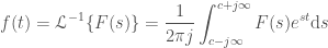

 to
to  , and
, and  giving:
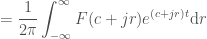

 “, but really it should be “Next two frequencies to add: … where
  ” since we are adding two frequencies at a time, in such a way that their imaginary parts cancel out, allowing us to keep everything real in the plots. I fixed this comment in the code, but didn’t want to rerender all the videos.
 . (A function that is 0 everywhere, except a sharp peak at exactly time = 0). In the S domain, this is a constant, meaning that we never converge. But visually it’s still cool.

