Why Kalman Filters are broken, and how to fix

Okay, so clickbait title, because I’m referring to the most common case of using a single Gaussian distribution to represent the current estimated position (for example) and for the measurement.

Here’s my problem with that:

They don’t take into account that sometimes things go wrong.

Now you may say ‘duh’, but it can cause some really serious problems if something does go wrong.

Say you have a self driving car. And the following happens:

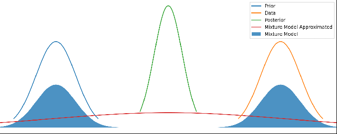
Prior: You currently estimate the position of a person in front of you to be at position: x = 2m ± 0.5m aka X ~ N(2,0.5)
Data: Your instruments return a new measure: the person is now measured to be at position: x = 10m ± 0.5m aka X ~ N(10,0.5)
Posterior: You apply your Kalman Filter and it concludes that the position of the person is now at: x = 6m ± 0.25m aka X ~ N(6,0.25)

gaussian1

You are now extremely confident that the person is at x=6m despite you previously thinking that they were at a x=2m and your measurement data says that they are at x=10m. You, the self driving car, now happily drive at x=10m.

How confident would you, as a, human, really be that the person is at x=6m? Barely at all, right? So something has gone wrong here.

Here’s an example in a simulator. A car is driving from right to left and we are trying to track its true position with a Extended Kalman Filter. ◯ The red circles indicate data from the simulated LASER, ◔ blue circle circles are RADAR, and ▲ green triangles are the position estimated by a Kalman filter. At the bottom of the arc, a single bad LASER data point is injected.

Credit to Udacity for the simulator.

The result is that the predicted position goes way off, and takes many times steps to recover.

The blame all lies on Sherlock Holmes:

sherlock

The product of N(2,0.5) * N(10,0.5) results in a ridiculous improbable scenerio – we have to scale up the result by $10^{14}$ . i.e. treating the highly improbable as truth. Perhaps what Sherlock should have said is that it is far more likely that you were simply mistaken in elimination! i.e. your prior or data was wrong!

Fixing the basic Kalman Filter

Here’s a small change we could make. We can add a small probability of ‘wtf’ to our system.

Prior: You currently estimate the position of a person in front of you to be at position: $x_{prior} = 2 \pm 0.5$ plus a $W_{prior}$ chance of ‘wtf’: aka: $X \sim (1-W_{prior}) \cdot N(2,0.5) + W_{prior} \cdot \textrm{WTF}$
Data: Your instruments return a new measure: the person is now measured to be at position: $x_{data} = 10 \pm 0.5$ plus a $W_{data}$ chance of ‘wtf’: aka:
$X \sim (1-W_{data}) \cdot N(10,0.5) + W_{data} \cdot \textrm{WTF}$
Posterior: You apply your bayes rule. What do we get now? We need the product of these two random variables, and then normalize, by setting C such that the total integral is 1. $\displaystyle{ \left( (1-W_{prior}) \cdot N(2,0.5) + W_{prior} \cdot \textrm{WTF} \right) \cdot \left( (1-W_{data}) \cdot N(10,0.5) + W_{data} \cdot \textrm{WTF} \right) / C}$ (note that $N(10,0.5) \cdot N(2,0.5)$ is proportionate to a new Gaussian scaled by a factor $S$ ) $= ( (1-W_{prior}) \cdot (1-W_{data}) \cdot N(6,0.25) \cdot S + (1-W_{prior}) \cdot W_{data} \cdot N(2,0.5) +$
$W_{prior} \cdot (1-W_{data}) \cdot N(10,0.5) + W_{prior} \cdot W_{data} \cdot \textrm{WTF}^2 ) / C$ We know that the area must equal 1 for a PDF, so we can determine the scale factor C. See Appendix below for any technical details, including the formula for S and C.So we have a solution, but the solution is a gaussian mixture model – a sum of a gaussian for the combination, a gaussian for the prior, and a gaussian for the data. So let’s simply pick the one with the highest probability, and roll the other two into the WTF weight.

Here’s the result as an gif – the posterior is where the posterior would normally be, and the shaded blue area is our ‘wtf’ version of the posterior as a weighted mixture model:

Various different priors and data. There’s no updating step here – just showing different mean values for the prior and data. The posterior is kept centered to make it easier to see.

It looks pretty reasonable! If the prior and data agree to within their uncertainties, then the mixture model just returns the posterior. And when they disagree strongly, we return a mixture of them.

Let’s now make an approximation of that mixture model to a single gaussian, by choosing a gaussian that minimizes the KL divergence.

Screenshot_20170726_015120

Which results in the red line ‘Mixture Model Approximated’:

Different priors and data, with the red line showing this new method’s output. As above, there’s no update step here – it’s not a time series.

Now this red line looks very reasonable! When the prior and data disagree with each other, we have a prediction that is wide and covers both of them. But when they agree with each other to within their uncertainties, we get a result that properly combines both and gives us a posterior result that is more certain than either – i.e. we are adding information.

In total, the code to just take a prior and data and return a posterior is this:
(Note: I’ve assumed there are no covariances – i.e. no correlation in the error terms)

# prior input
mu1 = 5
variance1 = 0.5
# data input
mu2 = 6
variance2 = 0.5
# This is what you would normally do, in a standard Kalman Filter:
variance3 = 1/(1/variance1 + 1/variance2)
mu3 = (mu1/variance1 + mu2/variance2)*variance3

#But instead we will do:
S = 1/(np.sqrt(2*np.pi*variance1*variance2/variance3)) * np.exp(-0.5 * (mu1 - mu2)**2 * variance3/(variance1*variance2))
Wprior = 0.01 # 1% chance our prior is wrong
Wdata = 0.01 # 1% chance our data is wrong
C = (1-Wprior) * (1-Wdata) * S + (1-Wprior) * Wdata + Wprior * (1-Wdata)
weights = [
Wprior * (1-Wdata) /C, # weight of prior
(1-Wprior) * Wdata /C, # weight of data
(1-Wprior) * (1-Wdata) * S/C ] #weight of posterior
mu4 = weights[0]*mu1 + weights[1]*mu2 + weights[2] * mu3
variance4 = weights[0]*(variance1 + (mu1 - mu4)**2) + \
weights[1]*(variance2 + (mu2 - mu4)**2) + \
weights[2]*(variance3 + (mu3 - mu4)**2)

So at mu3 and variance3 is the green curve in our graphs and is the usual approach, while mu4 and variance4 is my new approach and is a better estimation of posterior.

The full ipython notebook code for everything produced here, is in git, here:

https://github.com/johnflux/Improved-Kalman-Filter/blob/master/kalman.ipynb

Results: Testing out in Simulator

Unfortunately, in my simulator my kalman filter has a velocity component, which I don’t actually take into in my analysis yet. My math completely ignores any dependent variables. The problem is that when we increase the uncertainty of the position then we also need to increase the uncertainty of the velocity.

To salvage this, I used just a small part of the code:

<div>
<div>double Scale = 1/(sqrt(2*M_PI*variance1*variance2/variance3)) * exp(-0.5 * (mu1 – mu2)*(mu1 – mu2) * variance3/(variance1*variance2));</div>
<div>
<div>
<div>if (Scale < 0.00000000001)
return; /* Just completely ignore this data point */</div>
</div>
</div>
</div>

The result is this:

Screenshot_20170802_012822

Appendix:

Just some technical notes, for completeness.

We can set $WTF = 1/(2A)$ where it can be anywhere between A and -A. We can take A to be large or even take the limit to infinity.
It is a Probability Density Function since the area is 1: $\int^A_{-A} 1/(2A) dx = 1$ , and can set the Cauchy principal value of the integral to be 1 to keep it a PDF in the limit.
$\int^A_{-A} \textrm{WTF}^2(x) dx \to 0$ since: $\int^A_{-A} 1/(2A)^2 dx = 2A/(4A^2) = 1/(2A)$ which tends to 0 as $A \to \infty$ .
The scale factor S is simple but tedious to calculate:
The scale factor C can then be calculated by just setting the integral to equal 1 since it’s a PDF: $C = (1-W_{prior}) \cdot (1-W_{data}) \cdot S + (1-W_{prior}) \cdot W_{data} + W_{prior} \cdot (1-W_{data})$

	John Tapsell on Nokia 6110 Part 3 –…
	Quackleb on Nokia 6110 Part 3 –…
	John Tapsell on Nokia 6110 Part 3 –…
	Quackleb on Nokia 6110 Part 3 –…
	Kale Solis on USB i2c convertor chip. A less…

John Tapsell

Director of Flux Programming Ltd – Available for hire! See 'About'!

Why Kalman Filters are broken, and how to fix

They don’t take into account that sometimes things go wrong.

Fixing the basic Kalman Filter

Results: Testing out in Simulator

Appendix:

Leave a Reply Cancel reply

They don’t take into account that sometimes things go wrong.

Fixing the basic Kalman Filter

Results: Testing out in Simulator

Appendix:

Share this:

Like this:

Leave a Reply Cancel reply