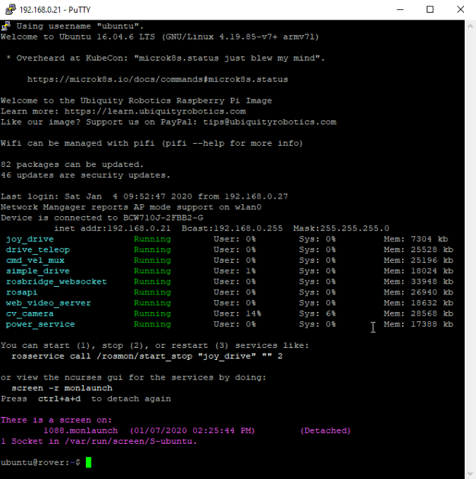
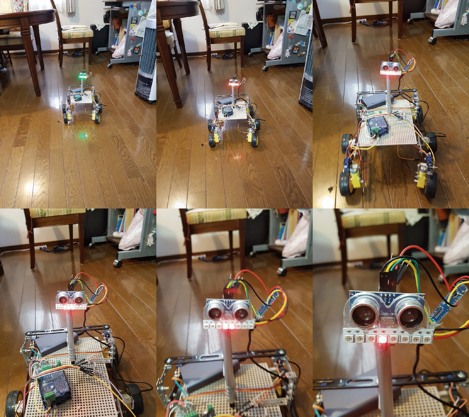
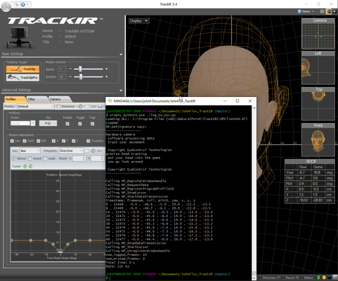
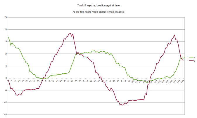
This is something that I’ve been working on for over 2 years now.
I’ve mentioned it before, but I thought I’d add some photos.
And we have the cameras hooked up to cool ‘robots’ / gantry systems:
This is something that I’ve been working on for over 2 years now.
I’ve mentioned it before, but I thought I’d add some photos.
And we have the cameras hooked up to cool ‘robots’ / gantry systems:
Heh, funny title.
I became interested in machine learning working for Nokia. I worked on Nokia’s Z Launcher application for Android. You can scribble a letter (or multiple), and it would recognize it and search for it. The app is available for download in the Play Store.
I worked on the Nokia Z Launcher’s handwriting recognition
Specifically I was tasked with optimizing the speed of the recognition. I don’t know if I can state any specifics on how the character recognition was done, but I will say that I managed to increase the speed of the recognition a hundred fold.
But this recognition was actually a relatively simple task, compared to modern day deep neural networks, but it really whet my appetite to understand more.
When Alpha Go beat Lee Sedol, I knew that I simply must understand Deep Neural Networks.
Below is my journey in understanding, along with my reflective thoughts:
Passed the Coursera Machine learning course with 97.6% score.
The lecturer, Andrew Ng, was absolutely awesome. My complaints, really, boil down to that I wish the course was twice as long and that I could learn more from him! I now help out in a machine learning chat group and find that most of the questions that people ask about TensorFlow, Theano etc are actually basics that are answered very well by Andrew Ng’s course. I constantly direct people to the course.
I needed to rename a whole load of files that were in Japanese. So I wrote a python program that translates the filename using google translate.
It’s not at all fancy, just run it and pass the filenames to translate and rename.
E.g.:
$ ls こんにちは世界.png $ sudo pip3 install googletrans $ translate_rename.py こんにちは世界.png こんにちは世界.png -> Hello_World.png $ ls Hello_World.png
#!/usr/bin/python3 import sys, re, os from googletrans import Translator translator = Translator() sourceLanguage = 'ja' destLanguage = 'en' # Set to false to actually rename the files dryRun = True def translate_and_rename(filename): filenameSplit = filename.rsplit('.',1) translated = translator.translate(filenameSplit[0], src=sourceLanguage, dest=destLanguage).text translated = re.sub( '[^a-zA-Z0-9.]+', '_', translated).strip().title() if len(filenameSplit) > 1: translated += '.' + filenameSplit[1] if filename == translated: print(filename, ' (unchanged)') else: print(filename, " -> ", translated) if not dryRun: os.rename(filename, translated) def main(argv): if len(argv) == 1: print("Need to pass filenames to translate and rename") for x in argv[1:]: translate_and_rename(x) if dryRun: print() print(" Dry run only - no actual changes made ") print() print("Edit this file and set DryRun to True") if __name__ == "__main__": main(sys.argv)
Maybe a clickbait title, sorry, but I couldn’t think of a better title.
The CPU ‘Meltdown’ bug affects Intel CPUs, and from Wikipedia:
Since many operating systems map physical memory, kernel processes, and other running user space processes into the address space of every process, Meltdown effectively makes it possible for a rogue process to read any physical, kernel or other processes’ mapped memory—regardless of whether it should be able to do so. Defenses against Meltdown would require avoiding the use of memory mapping in a manner vulnerable to such exploits (i.e. a software-based solution) or avoidance of the underlying race condition (i.e. a modification to the CPUs’ microcode and/or execution path).
This separation of user and kernel memory space is exactly what I worked on from 2012 to 2014 on behalf on Deutsch Telekom using the L4 hypervisor:
The idea was to give each service its own separate memory space, designing in a way such that you assume that the main OS has been compromised and is not trustworthy (e.g. because of the Meltdown bug). I personally worked on the graphics driver – splitting the kernel graphics driver into two parts – one side for the app to talk to and has to be considered compromised, and one side that actually talks to the hardware.
Here’s my work in action:
Yes, I did actually use Angry Birds as my test. Fully hardware accelerated too 🙂
Unfortunately the problem was that it took too long to port each phone across. It took me a year to port across graphics driver changes, and a similar time for my colleagues to do the other drivers. And then another year for it to actually hit the market. The result is that the phone was always over 2 years out of date by the time it hit the market, which is a long time in mobile phone times.
Still, our software would be immune to this type of bug, and that’s kinda cool. Even if it did fail commercially 😉
I love TypeScript. I use it whenever I can. That said, sometimes it can be… interesting. Today, out of the blue, I got the typescript error in code that used to work:
[06:53:30] typescript: src/mycode.ts, line: 57 Property 'video' does not exist on type 'number | (<U>(callbackfn: (value: Page, index: number, array: Page[]) => U, thisA...'. Property 'video' does not exist on type 'number'.
The code looks like:
return _.chain(pages) .filter((s, sIdx) => s.video || s.videoEmbedded) .map((s, sIdx) => { if (s.video) { ... }
Can you spot the ‘error’?
The problem is that s.video || s.videoEmbedded isn’t returning a boolean. It’s return a truthy value, but not a boolean. And the lodash typescript developers made a change 1 month ago that meant that filter() would only accept booleans, not any truthy value. And the lodash typescript developers are finding that fixing this becomes very complicated and complex. See the full conversation here:
https://github.com/DefinitelyTyped/DefinitelyTyped/issues/21485
(Open issue at time of writing. Please leave me feedback or message me if you see this bug get resolved)
The workaround/fix is to just make sure it’s a boolean. E.g. use !! or Boolean(..) or:
return _.chain(pages) .filter((s, sIdx) => s.video !== null || s.videoEmbedded !== null ) .map((s, sIdx) => { if (s.video) { ... }
Just a light hearted post today. My daughter had a great idea to build a felt house for her teddy cat, so we did it together.
It was a fun project, and simple to make. The wood is just children’s blocks glued together, and the felt is stapled on. The strap was cut from an ecobag. A piece of velcro was added to hold the door open.
I’ve implemented PID control far too many times now, and I’ve never been that happy with the results.
It is simple to implement, but tricky to tune. My thick control theory book says that 95% of commercial in-use PID systems are sub-optimally tuned. And I can believe it.
I’ve been recently playing with other systems, and currently I really like Model Predictive Control. It does require some significant compute power, which was a big problem when it was invented, but not so much any more. (As a side point, I’d like to implement MPC in tensorflow. That would be cool, and could probably be done in a weekend).
I wrote a PID control system for a self driving car. It is dumbly auto-tuned, so to speak, by a simple twiddle method. It tests out a particular set of PID values for one minute, resets the track, then picks a new set of PID values based on the best seen values, changed slightly.
The results are… very underwhelming.
The same driving but using Model Predictive Control, below, starts to look a lot nicer. For reference, the PID control took a total of two days to implement, and the MPC took a total of three days. The MPC version also has an additional complication – there’s a simulated delay of 100ms.
But I’m very pleased with the results. It’s a bit jerky here due to random latency variations, made worse by the screen recording software. I’ve got some ideas on trying to solve that by timestamping, but I don’t think I’ll have time to work on it.
I would love to try applying this MPC system to a Quadcopter. I’ve written quite a bit previously about latency problems with PID in a quadcopter: (In this video, the ufo-shaped quadcopter is attempting to move to, and maintain, a fixed position above the chair. Ignore the blue man 🙂 )
Okay, so clickbait title, because I’m referring to the most common case of using a single Gaussian distribution to represent the current estimated position (for example) and for the measurement.
Here’s my problem with that:
Now you may say ‘duh’, but it can cause some really serious problems if something does go wrong.
Say you have a self driving car. And the following happens:
How confident would you, as a, human, really be that the person is at x=6m? Barely at all, right? So something has gone wrong here.
Here’s an example in a simulator. A car is driving from right to left and we are trying to track its true position with a Extended Kalman Filter. ◯ The red circles indicate data from the simulated LASER, ◔ blue circle circles are RADAR, and ▲ green triangles are the position estimated by a Kalman filter. At the bottom of the arc, a single bad LASER data point is injected.
Credit to Udacity for the simulator.
The result is that the predicted position goes way off, and takes many times steps to recover.
The blame all lies on Sherlock Holmes:
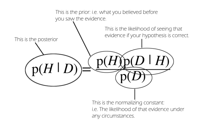
The product of N(2,0.5) * N(10,0.5) results in a ridiculous improbable scenerio – we have to scale up the result by . i.e. treating the highly improbable as truth. Perhaps what Sherlock should have said is that it is far more likely that you were simply mistaken in elimination! i.e. your prior or data was wrong!
Here’s a small change we could make. We can add a small probability of ‘wtf’ to our system.
Here’s the result as an gif – the posterior is where the posterior would normally be, and the shaded blue area is our ‘wtf’ version of the posterior as a weighted mixture model:
Various different priors and data. There’s no updating step here – just showing different mean values for the prior and data. The posterior is kept centered to make it easier to see.
It looks pretty reasonable! If the prior and data agree to within their uncertainties, then the mixture model just returns the posterior. And when they disagree strongly, we return a mixture of them.
Let’s now make an approximation of that mixture model to a single gaussian, by choosing a gaussian that minimizes the KL divergence.
Which results in the red line ‘Mixture Model Approximated’:
Different priors and data, with the red line showing this new method’s output. As above, there’s no update step here – it’s not a time series.
Now this red line looks very reasonable! When the prior and data disagree with each other, we have a prediction that is wide and covers both of them. But when they agree with each other to within their uncertainties, we get a result that properly combines both and gives us a posterior result that is more certain than either – i.e. we are adding information.
In total, the code to just take a prior and data and return a posterior is this:
(Note: I’ve assumed there are no covariances – i.e. no correlation in the error terms)
# prior input mu1 = 5 variance1 = 0.5 # data input mu2 = 6 variance2 = 0.5 # This is what you would normally do, in a standard Kalman Filter: variance3 = 1/(1/variance1 + 1/variance2) mu3 = (mu1/variance1 + mu2/variance2)*variance3 #But instead we will do: S = 1/(np.sqrt(2*np.pi*variance1*variance2/variance3)) * np.exp(-0.5 * (mu1 - mu2)**2 * variance3/(variance1*variance2)) Wprior = 0.01 # 1% chance our prior is wrong Wdata = 0.01 # 1% chance our data is wrong C = (1-Wprior) * (1-Wdata) * S + (1-Wprior) * Wdata + Wprior * (1-Wdata) weights = [ Wprior * (1-Wdata) /C, # weight of prior (1-Wprior) * Wdata /C, # weight of data (1-Wprior) * (1-Wdata) * S/C ] #weight of posterior mu4 = weights[0]*mu1 + weights[1]*mu2 + weights[2] * mu3 variance4 = weights[0]*(variance1 + (mu1 - mu4)**2) + \ weights[1]*(variance2 + (mu2 - mu4)**2) + \ weights[2]*(variance3 + (mu3 - mu4)**2)
So at mu3 and variance3 is the green curve in our graphs and is the usual approach, while mu4 and variance4 is my new approach and is a better estimation of posterior.
The full ipython notebook code for everything produced here, is in git, here:
https://github.com/johnflux/Improved-Kalman-Filter/blob/master/kalman.ipynb
Unfortunately, in my simulator my kalman filter has a velocity component, which I don’t actually take into in my analysis yet. My math completely ignores any dependent variables. The problem is that when we increase the uncertainty of the position then we also need to increase the uncertainty of the velocity.
To salvage this, I used just a small part of the code:
<div>
<div>double Scale = 1/(sqrt(2*M_PI*variance1*variance2/variance3)) * exp(-0.5 * (mu1 – mu2)*(mu1 – mu2) * variance3/(variance1*variance2));</div>
<div>
<div>
<div>if (Scale < 0.00000000001)
return; /* Just completely ignore this data point */</div>
</div>
</div>
</div>
The result is this:
Just some technical notes, for completeness.
For my self-driving car, I detect cars in the image by scanning over the image in windows of varying sizes, and use the detection results to build up a ‘heat map’ of the most likely areas for where the cars are.
For visualization I came up with this idea:
In code:
heat_img = plt.cm.hot(heat/np.max(heat)) heat_img[heat<1,3] = 0 image2 = np.copy(image) image2[heat>1,:] = image2[heat>1,:]/3 + (heat_img[heat>1,0:3]*256*2/3).astype(np.uint8) plt.imshow(image2)
Well, in a simulator 🙂
(Sorry about the bad filming – it was the easiest way to get even a semi-decent quality)
Code is here: https://github.com/johnflux/CarND-Behavioral-Cloning-P3
I basically follow the NVidia End to End Learning for Self-Driving Cars paper with a few tweaks to add in dropout, slightly larger Dense layers to compensate, and an additional convolution layer to handle the different input image resolution. It runs in real time on a GTX 980 Ti.