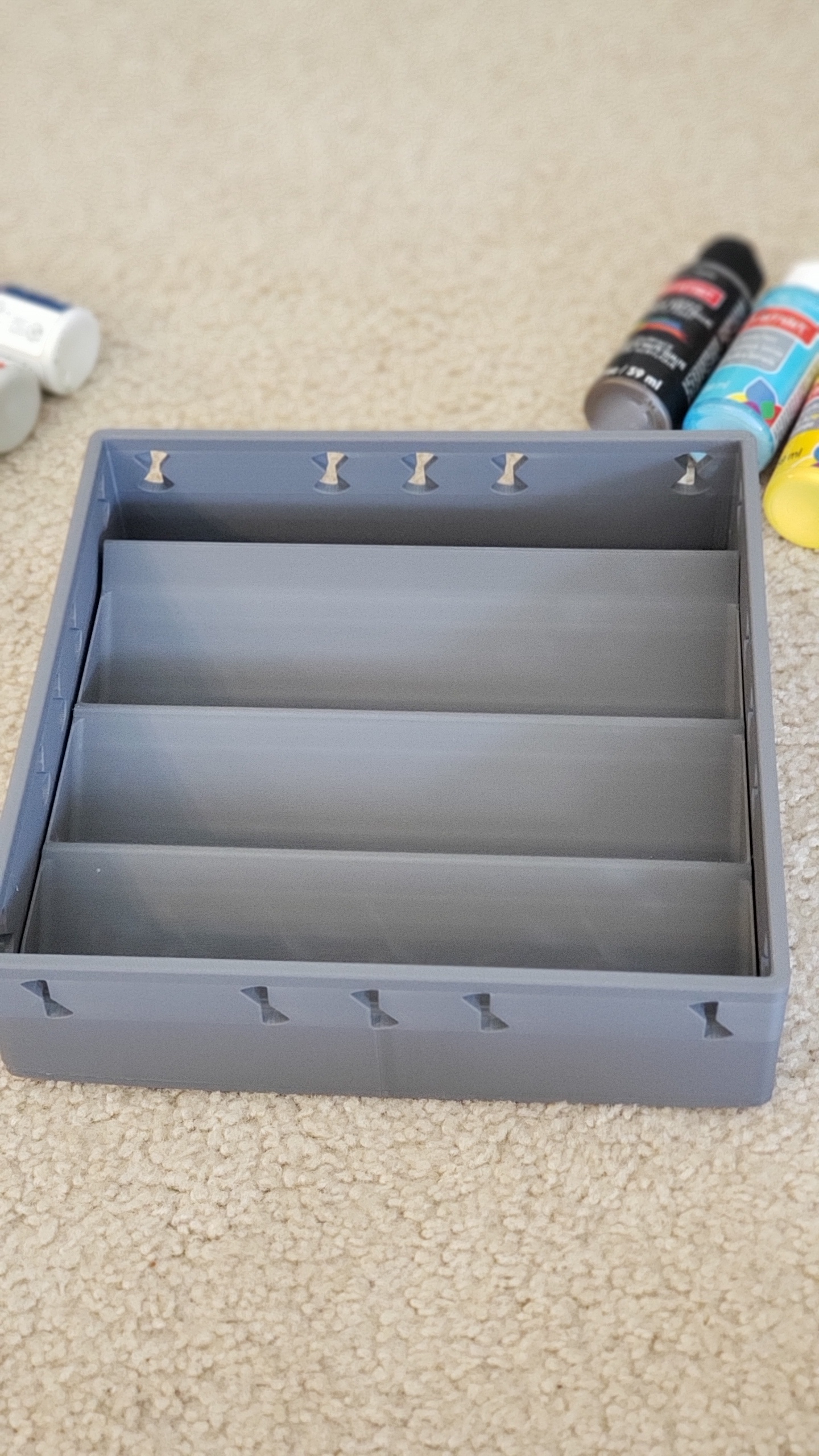
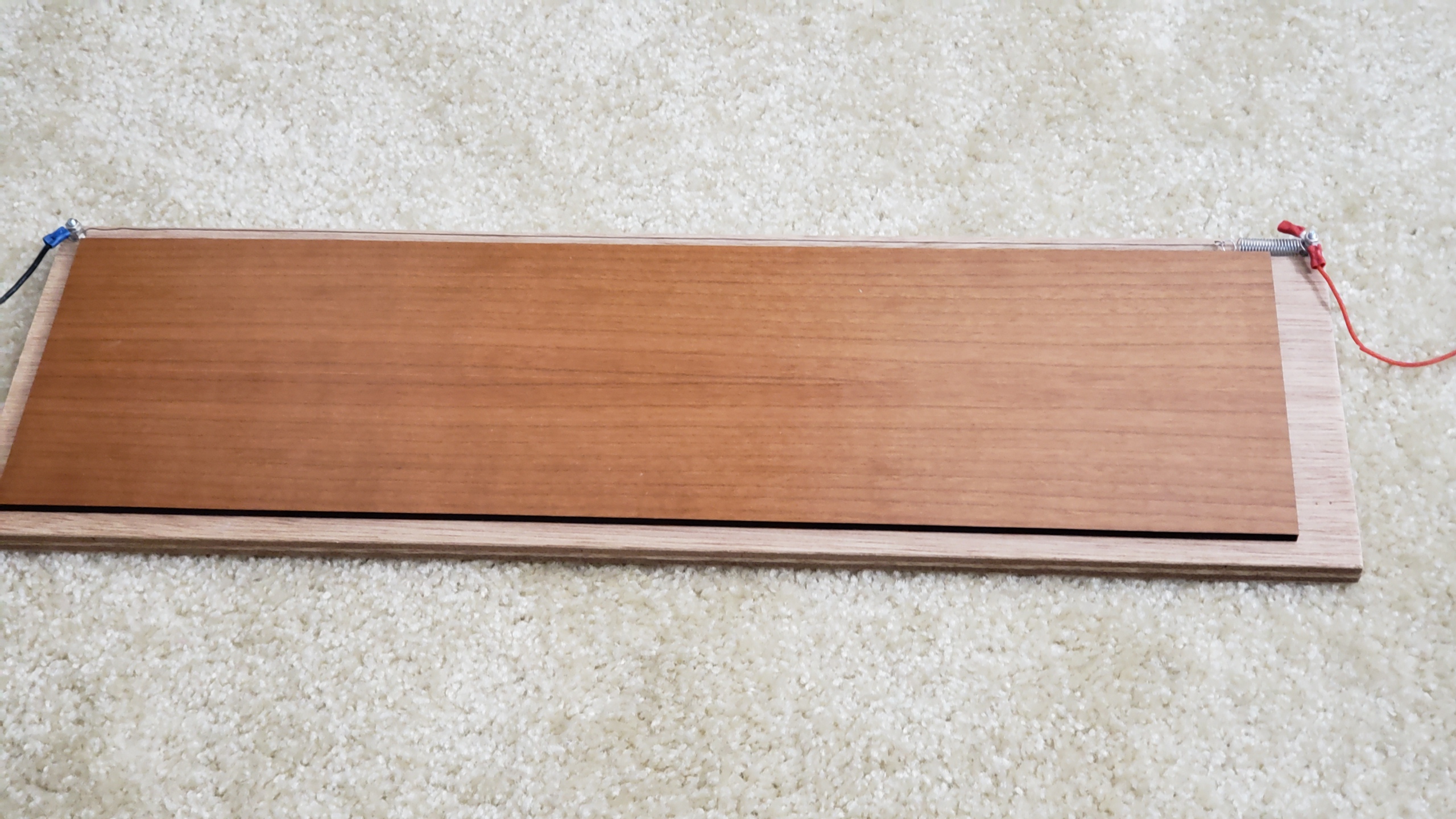
I wanted to hold some paints in a box. Pretty simple requirement, but nicely demonstrates my process in creating something.
Crude mock-ups
I find this is one of the most important steps. When thinking just in my head, or even on paper or in CAD, it’s really easy to lose sense of scale and proportions and miss really obvious things like whether paints would even be removable etc. You don’t want to go through the whole process and then realize at the end up that there’s no actual way to grab a paint etc. Having something physical, I find, helps to get my mind find creative solutions.
It did pay off. I had expected that being at an angle would be a huge waste of space, but in my particular setup it would take 2 trays with height 120mm, to pack all the paints vertically with no space between them, so a total height of 240mm. Whereas if they are lying at angle it would take 3 trays, but with a height of 90mm so a total of 270mm. So only 12.5% higher. 12.5% higher in return for the advantage of being able to actually see the paints is well worth it for me.
Calculate on paper
Might not be necessary, but I enjoy the process of just playing with stuff on paper, and solving constraints by hand can give me a better intuition for what the limiting factors are.
Solidworks
Transfer that to Solidworks, keeping in mind that 3D printers want fillets on the top and chamfers on the bottom, and materials don’t want sharp angles.
Note my tolerances are super tight. The height needs to be less than 85mm to fit in the box I have – which is 90mm height, with a 5mm bottom. In this drawing it is 84.86mm. To strengthen the 1.2mm floor, I added 1mm walls on both sides. Thin, but again the tolerances are very tight and I don’t have any more than 2mm total to spare.
Use mirror features etc to make it easier to maintain and adjust later. Note the fillets to strengthen the walls.
And fillet everything, to reduce strain on the material and to give it a more professional feel. Noone wants sharp corners:
And render it, just for vanity 🙂
3D Print
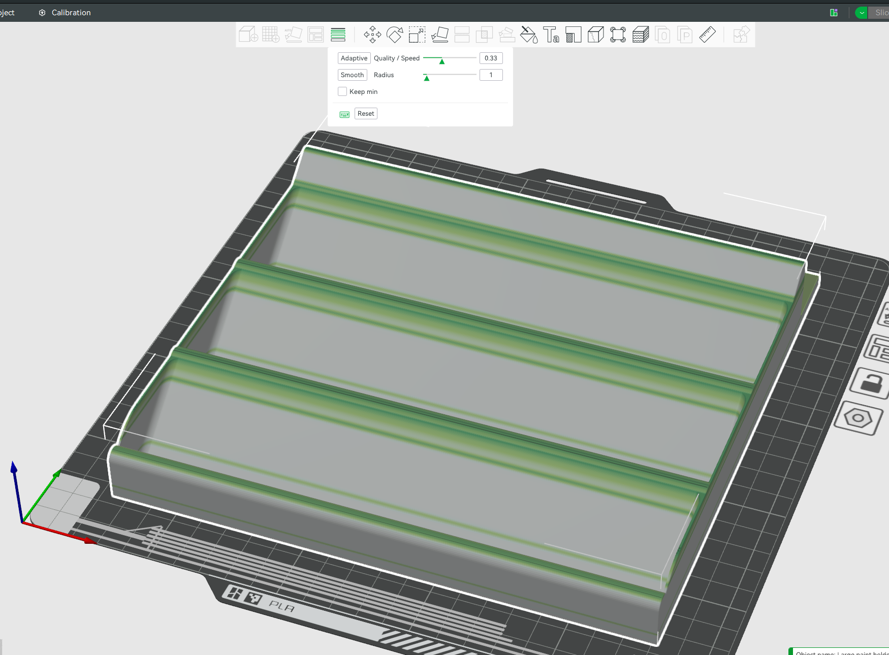
In Bambulabs, I love the variable layer height. Print all the solid parts fast, and then slow down just for the tops. Adds only 10 minutes to the print, in return for high quality curves.
This article is just me playing about with math, and showing how to extrapolate in ways that might not be immediately obvious, looking at how much AI can memorize chess
Summary
The Licess chess database has 5 billion chess games recorded. There is no evidence of us even scratching the surface of unique chess games. Games are really unique. Even if an AI memorized all 5 billion games, it would help for approximately 4 moves, and then the game would be unique
Background
In 2019, the lichess chess database had 500 million games recorded.
In those games, as of 2019, there were 21.5 billion unique positions, and 76% of all positions were unique. So a game had an average of 32 unique positions. A chess game has only 34-35 moves on average, so any given game is going to start being unique in only a few moves!
But as of writing in Nov 2023, the lichess chess database now has almost exactly ten times more games. Can we extrapolate how many unique positions it has now?
Power Law Approximation (Similar games are rare, but happen occasionally)
It’s not something we can answer without more data, but a reasonable starting point with the assumption that similar games are rare but happen occasionally, is a power law of approximately 0.5. Since we have 10 times more chess games, we can expect approximately sqrt(10) more unique positions, so ~68 million unique board positions in 2014 in 5 billion games.
Logarithmic Approximation (Similar games happen often)
As a conservative lower limit for this curve, we could instead fit logarithmic decay curve, instead of power law, to this using two data points:
1 game corresponds to 35 unique positions.
500 million games correspond to 21.5 billion unique positions.
So we want to solve:
35 = a log(b + 1) 21,500,000,000 = a log(b * 500000000 + 1)
But Wolfram Alpha timed out trying to solve it.
In python, solve and nsolve failed to solve it, but least_squares cracked it:
from scipy.optimize import least_squares
import numpy as np

# Define the function that calculates the difference between the observed and predicted values
def equations(p):
    a, b = p
    eq1 = a * np.log(b * 1 + 1) - 35  # Difference for the first data point
    eq2 = a * np.log(b * 500_000_000 + 1) - 21_500_000_000  # Difference for the second data point
    return (eq1, eq2)

bounds = ([1, 0], [np.inf, 1])


# Initial guesses for a and b
initial_guess = [10000, 1e-8]

# Perform the least squares optimization
result = least_squares(equations, initial_guess, bounds=bounds)

a_opt, b_opt = result.x
cost = result.cost

# Check the final residuals
residuals = equations(result.x)

print(f"Optimized a: {a_opt}")
print(f"Optimized b: {b_opt}")
print(f"Residuals: {residuals}")
print(f"Cost: {cost}")
Gives me: 1757372725 log(0.000411370x + 1)
Which gives ~25 billion unique board positions in 2023 for the conservative lower bound. (See summary for more)
New Data Point found! Lichess Opening Explorer
Lichess released an opening explorer – 12 million chess games, with 390 million unique positions. This gives us a new data point to test which model fits. This is what we have so far:
Let’s zoom in and see which model the lichess opening explorer fits:
The linear model! This means that the database of 5 billion games does not even scratch the surface of the 10^44 possible board positions in any way that we can detect…. although written like that it’s kinda obvious tbh.
Summary and interpretation
In the 2019 Lichess chess database, there were 500 million games, and 75% of game positions were unique,
In the 2023 Lichess chess database, there are 10 times as many games, and so extrapolating:
There are ~68 billion unique board positions using a power scaling law of 0.5. This is an empirical guess which models what we frequently see in nature. With 5000 million games and 35 moves per game, this means that only 0.4% of board positions are unique, and only 1.4% of games have a board position that hasn’t been played before.
There are ~25 billion unique board positions using a conservative lower bound estimate using logarithmic scaling). With 5000 million games and 35 moves per game, this means that only 0.14% of board positions are unique, and only 0.5% of games have a board position that hasn’t been played before.
If a board position can be stored in an average of 8 bytes (64 bits) then this could be stored in 1.4 GB. So easily fit in an over-fitted trained AI. But there are 10^44 possible board combinations. There is no evidence that we are even scratching the surface of being able to memorize
Conclusion: AI could memorize the entire 5 billion chess games, and it wouldn’t help. Probably.. see caveat
Caveat
This whole thing was kinda of a joke, and there’s one big serious flaw with the final conclusion. If the AI plays a move from the database, that’s no longer a random sampling of a game from the database, and the chance of a similar game being played goes way up. But in a way I can’t model. Oh well.
Edit: User Wisskey pointed out that, among other mistakes that I’ve made and fixed, that:
A move in chess corresponds to moves (actually called plies instead of moves) by both sides, so 1 move = 2 chess positions, not 1 chess position.
User: Wisskey
So, I’m probably off by a factor of 2 in places, not that it’s going to matter much to the final conclusion
I’ve been working on an open source ChatGPT clone, as a small part of a large group:
There’s me – John Tapsell, ML engineer 🙂 Super proud to be part of that amazing team!
Open Assistant is, very roughly speaking, one possible front end and data collection, and RWKV is one possible back end. The two projects can work together.
I’ve contributed a dozen smaller parts, but also two main parts that I want to mention here:
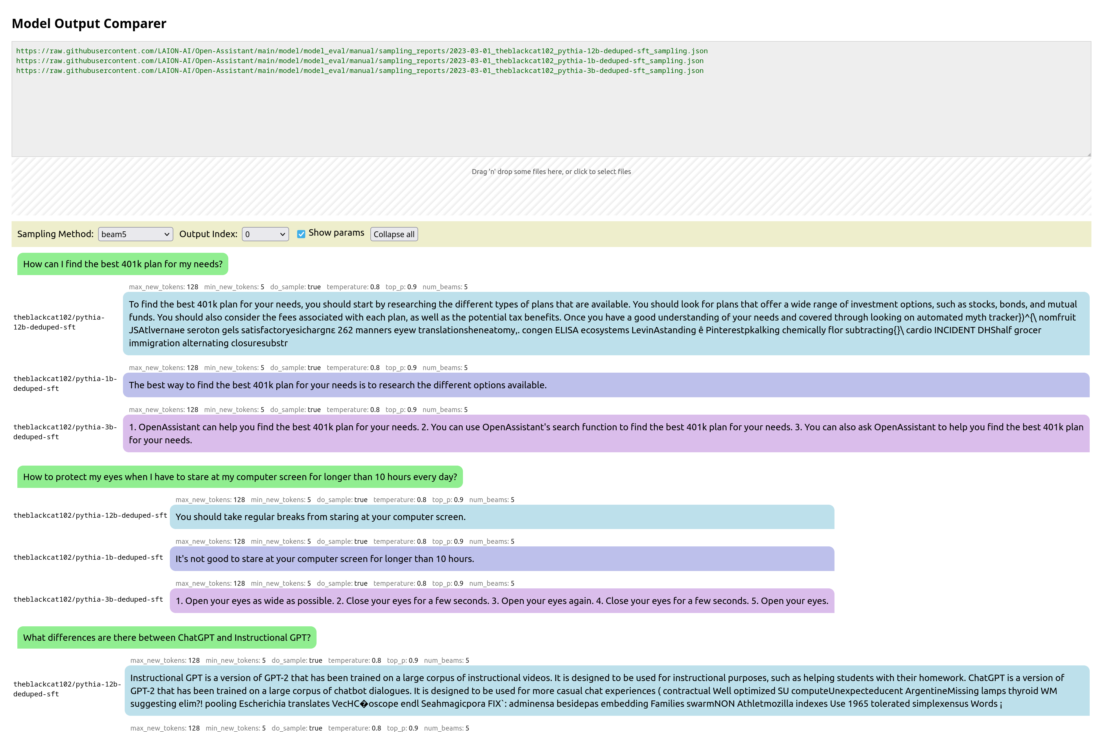
React UI for comparing the outputs of different models, to compare them. I call it: Open Assistant Model Comparer!
Different decoding schemes in javascript for RWKV-web – a way to run RWKV in the web browser – doing the actual model inference in the browser.
Open Assistant Model Comparer
This is a tool I wrote from scratch for two open-source teams: Open Assistant and RWKV. Behold its prettiness!
You pass it the urls of json files that are in a specific format, each containing the inference output of a model for various prompts. It then collates these, and presents them in a way to let you easily compare them. You can also drag-and-drop local files for comparison.
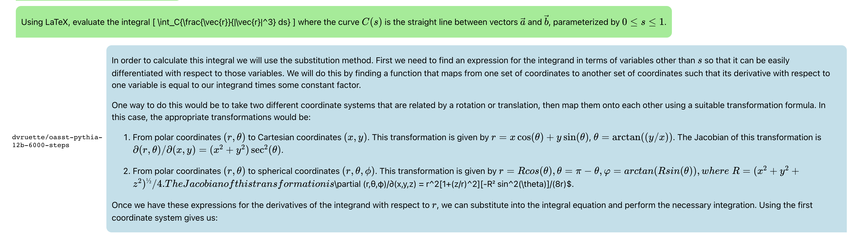
Update: Now with syntax highlighting, math support, markdown support,, url-linking and so much more:
And latex:
and recipes:
Javascript RWKV inference
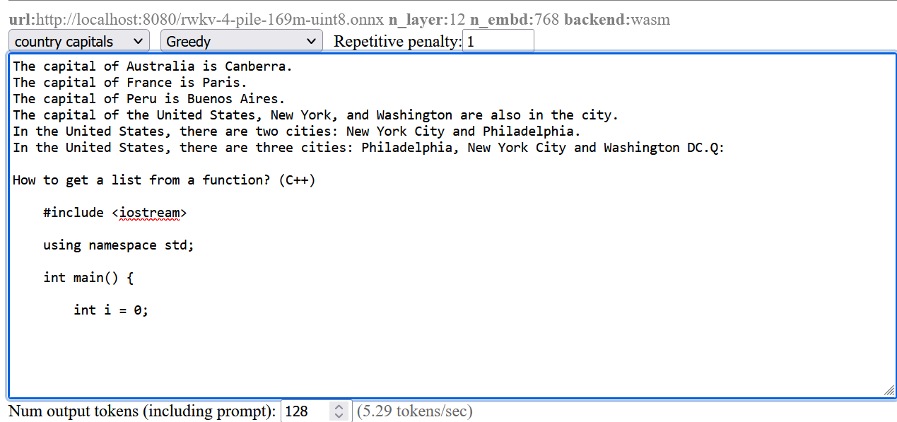
This is an especially cool project. RWKV is a RNN LLM. A guy in the team, josephrocca, got it running in the browser, as in doing the actual inference in the browser, by running the python code in Wasm (WebAssembly).
I worked on cleaning up the code, and making it a library suitable for other projects to use.
When we run inference on a model, at each step the model is providing confidence values for each token, and from those confidence values we pick a particular token, before repeating for the next token.
We could pick token with the highest confidence, aka greedy search. But this has various downsides – we will never pick tokens that are also valid (and perhaps more rarer and more interesting), and in smaller LLM results in very repetitive output.
I implemented some alternatives:
multinomial sampling. Take the top few more confident outputs, apply a softmax and normalize to produce probabilities, then treat them as probabilities and sample from them. We can apply a temperature, to make lower-probable results more or less likely.
Repetitive penalty. We can explicitly look back at the tokens that we’ve generated so far, and penalize similar tokens to make them less likely to appear again.
The result:
The screenshots are from a pretty small model. Here’s a comparison from a larger RWKV (RL LLM) model:
Greedy (no penalty):
"The system of education in the present day world is not satisfactory, it is a system of totalitarianism, it is a system of oppression, it is a system of exploitation, it is a system of exploitation of the people, it is a system of exploitation of the people by the people, it is a system of exploitation of the people by the government, it is a system of exploitation of the people by the government...(repeated text)"
Greedy+Repetition penalty:
"The system of education in the present day world is not satisfactory, it is a system of totalitarianism. The system of modern education is based on the theory of class struggle and the aim of this theory is to control and enslave people. The purpose of this system is to make people submissive and docile. It makes them accept all kinds of injustices, crimes and atrocities as normal conditions. It forces people to accept their own degradation as a result of their own acts. This kind of mentality makes it impossible for any person to think independently, for him to be critical about his own condition, his environment or his culture. "
Sampling top-p=0.8 temperature=1:
"and say something about schools and their role in today's world. I will try to show there are shortcomings in both the system and people. Some flaws of the system are as follows: There are many unruly and disobedient people, especially males, who cannot be controlled. It is impossible for those who lack common sense and insight to appreciate the significance of any decision made with a view to the overall good, such as the deployment of new technologies and machinery. Uneducated persons cannot make the right decisions. They do not value authority, obedience to the law and societal traditions, and they do not feel that these moral
Most people preferred the Greedy + Repetition penalty output.
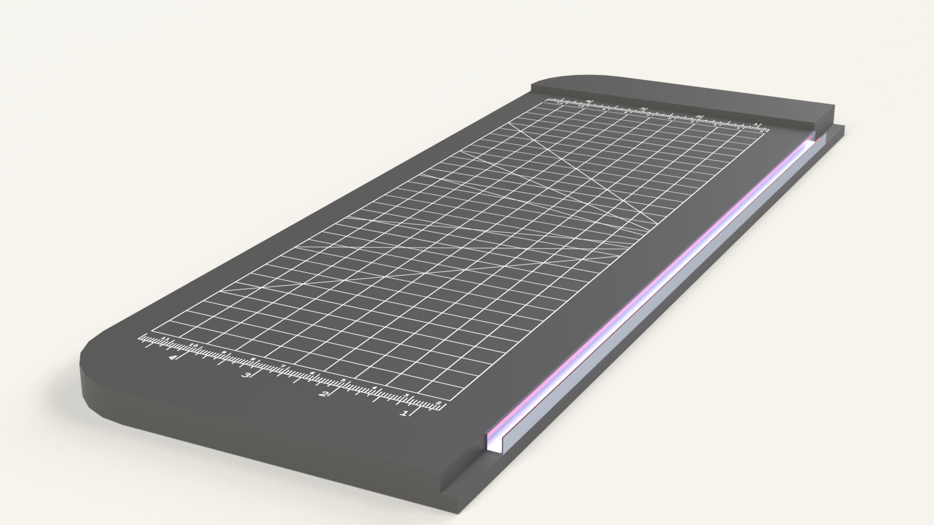
I wanted to laser cut acrylic plastic, and then bend it into shapes.
So I mocked something up:
(The pink glow was my attempt to render a glow hot wire)
It’s extremely simple. It’s just a base and a channel along one edge with a nichrome wire (the wire used in e-cigarettes).
I actually built 5 of these, in different styles, methods and sizes.
And here’s a version built:
Here you can see how the wire is secured. It wraps around two bolts, and held in place with nuts. One end is connected to a spring because the wire shrinks as the wire gets hot.
I apply 12V across the wire, wait a minute for it to become hot, then place a piece of acrylic across the wire, wait a few seconds for it to become soft, then bend.
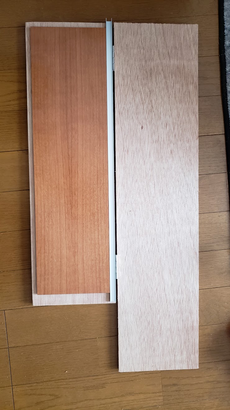
Folding version
Out of the five I built, three of them used a second piece with a hinge, like below, and also used an actual metal channel. My thinking is that I would heat up the plastic, hold it in place, then bend it smoothly with the second piece. However I found that I never used the hinge – it was far easier to just bend against the table or bend it around a piece of wood etc
Example
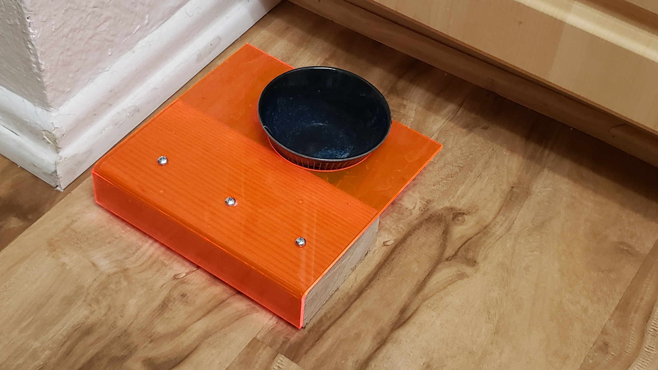
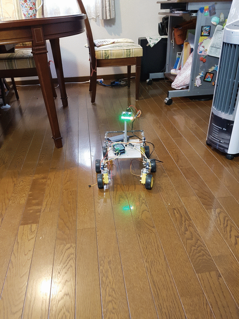
The main use was to bend the casing for my wire bender and mars rover, but these aren’t done yet.
So here’s a cat’s water bowl holder that I made, by bending acrylic around a 2×4 block. I laser cut a circle first to allow the water bowl to fit.
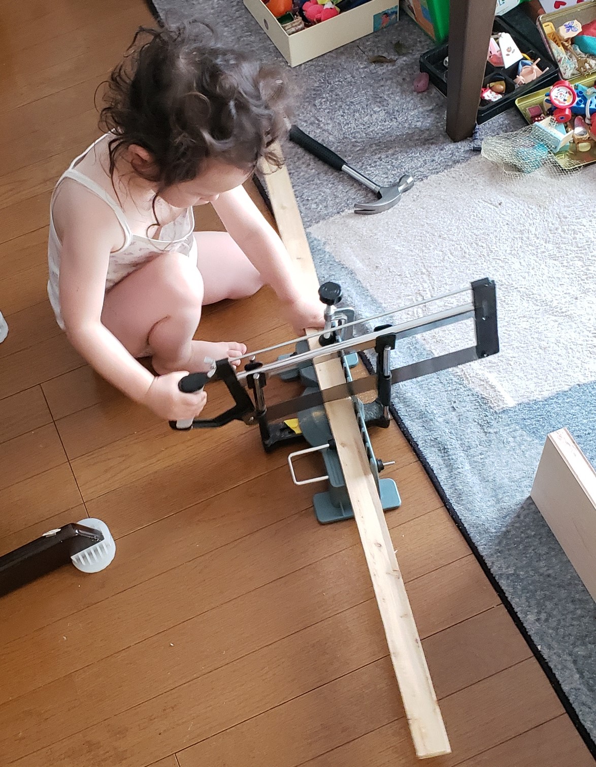
Fast development
The real key to fast development is outsourcing the hard work:
My daughter loved this ‘Flamingo’ song on youtube, so I laser cut out the ‘shrimp’ in wood, acrylic and pink paper, then mounted them together with an android tablet all inside of a frame. The result was pretty cool imho. (Unfortunately I can’t show the full thing for copyright reasons.)
This is an ongoing multi-year project. I need to write this up properly, but I’ve got so much stuff that I’m going to attack this in stages.
Current Status
14 motors, controlled by a raspberry pi. Arm doesn’t quite work yet. Everything else works.
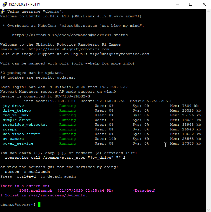
Front end – I wrote this in ReactJS, and it communicates with the robot via a websocket to RobotOS, using ‘rosbridge’. Sorry it’s so pink – it uses infrared LEDs to work at night, but they are kinda overpowering. Also sorry for the mess – I have two children…
In the top left, the green circle is a ‘nipple’ – to let you move the rover about via webpage. Either via mouse or finger press.
In the top right, the xbox controller image shows what buttons are being pressed on an xbox controller, to control the robot. The xbox controller can either be connected to the rover, or connected to the PC / mobile phone – the webpage relays controller commands through to the rover.
Beneath the xbox controller is the list of running processes (“ros nodes”), with cpu and mem information.
Below that is the error messages etc.
Console UI
I’m strong believer in trying to make my projects ‘transparent’ – as in, when you connect, it should be obvious what is going on, and how to do things.
With that in mind, I always create nice colored scripts that show the current status.
Below is the output when I ssh into the raspberry pi. It shows:
– Wifi status and IP address
– Currently running ROS Node processes, and their mem and cpu status. Colored Green for good, Red for stopped/crashed.
– Show that ‘rosmon’ is running on ‘screen’ and how to connect to it.
– The command line shows the current git status
See those links for the source code. I think that every ROS project can benefit from these.
Boogie Rocker Design
Ultrasonic Sensor
I played about with making a robot face. I combined a Ultrasonic Sensor (HC-SR04) and NeoPixel leds. The leds reflect the distance – one pixel per 10 of cm.
I’m wondering if I can do SLAM – Simultaneous Location And Mapping with a single (or a few) very-cheap ultrasonic sensor. Well, the answer is almost certainly no, but I’m very curious to see how far I can get.
NOTE: This is an old design – from more than two years ago
I wanted a simple way to track the movement and orientation of an object (In this case, my Samurai robot). TrackIR’s SDK is not public, and has no python support as far as I know.
I looked at the symbols in dll that is distributed with the trackir app, and with some googling around on the function names, I could piece together how to use this API.
Here’s the result – my console program running in a window in the middle. I have pressed ctrl+c after 70ms, to cancel, to give a better screenshot:
Implementation Details
Python lets you call functions in any .dll library pretty easily (although the documentation for doing so is pretty awful). The entire code is approximately 500 lines, with half of that being comments, and I’ve put on github here:
Query the Windows registry for where the TrackIR software is installed.
Load the NPClient64.dll in that TrackIR software folder, using python ctypes.WinDLL (Note, I’m using 64 bit python, so I want the 64 bit library)
Expose each function in the dll that we want to use. This can get a bit cryptic, and took a bit of messing about to get right. For example, there is a function in the dll ‘NP_StopCursor’, that in C would look like:
where ‘NP_StopCursor’ is now a function that can then be called with: NP_StopCursor(). See the trackir.py file for more, including on how to pass parameters which are data structures etc.
Note: Python ctypes supports a way to mark a parameter as an ‘output’, but I didn’t fully understand what it was doing. It seemed to just work, and appeared to automatically allocate the memory for you, but the documentation didn’t explain it, and I didn’t entirely trust that I wasn’t just corrupting random memory, so I stuck to making all the parameters input parameters and ‘new’ing the data structure myself.
Create a graphical window and get its handle (hWnd), and call the functions in the TrackIR .dll to setup the polling, and pass the handle along. The TrackIR software will poll every 10 seconds ish to check that the given graphic window is still alive, and shutdown the connection if not.
Poll the DLL at 120hz to get the 6DOF position and orientation information.
ROS Integration
I wanted to get this to stream 6DOF data to ROS as well, to open up possibilities such as being able to determine the position of a robot, or to control the robot with your head etc.
The easiest way is to run a websocket server on the linux ROS server, and send the data via ROS message via the websocket.
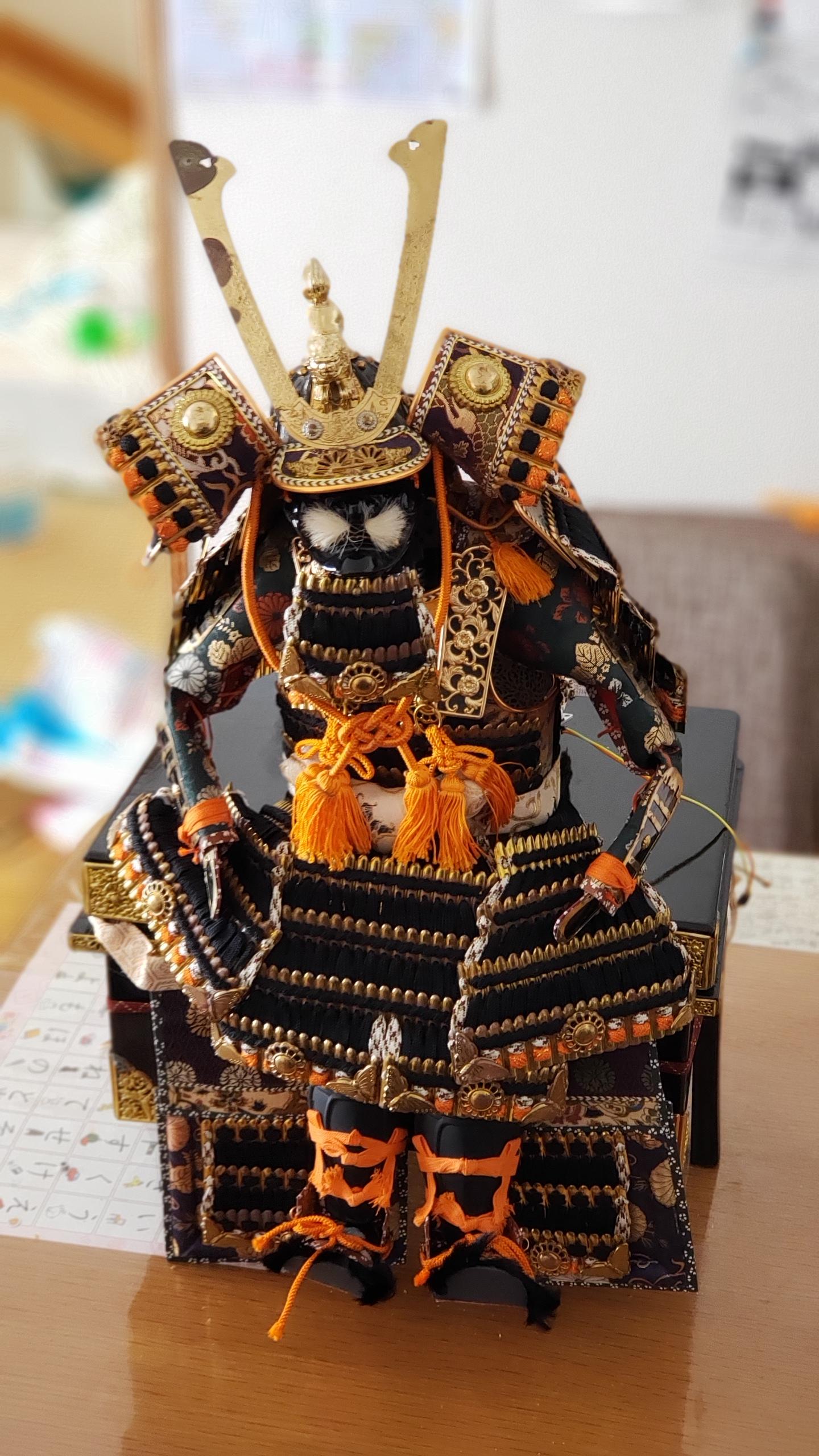
I saw this for sale in a Christmas market for 500 yen (~$5 USD) and immediately bought it. My friends questioned my sanity, since it’s for “boy’s day” (It’s a “五月人形”) and we have no boys.
But, I could see the robotic potential!
Note: I have put the gold plated metal through an ultrasonic cleaner and buffed them with British Museum wax. But I’m not sure how to remove the corrosion – please message me if you have any ideas.
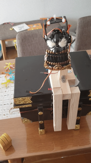
Next step is to build a wooden skeleton to mount the motors:
I’ve used 2 MG996 servo motors (presumably clones).
And a quick and dirty arduino program to move the head in a circular motion:
#include
Servo up_down_servo; // create servo object to control a servo
Servo left_right_servo; // create servo object to control a servo
int pos = 0; // variable to store the servo position
void setup() {
up_down_servo.attach(8); // attaches the servo on pin 8 to the servo object
up_down_servo.write(170); // Maximum is 170 and that's looking forward, and smallest is about 140 and that is looking a bit downwards
left_right_servo.attach(9); // attaches the servo on pin 9 to the servo object
left_right_servo.write(170); // 155 is facing forward. 170 is looking to the left for him
Serial.begin(115200);
Serial.println("up_down, left_right"); // Output a CSV stream, showing the desired positions
}
void loop() {
const float graduations = 1000.0;
for (pos = 0; pos < graduations; pos++) {
const float up_down_angle = 160+10*sin(pos / graduations * 2.0 * 3.1415);
const float left_right_angle = 155+5*cos(pos / graduations * 2.0 * 3.1415);
left_right_servo.write(left_right_angle);
up_down_servo.write(up_down_angle);
Serial.print(up_down_angle);
Serial.print(",");
Serial.println(left_right_angle);
delay(15);
}
}
And the result:
Jerky Movement
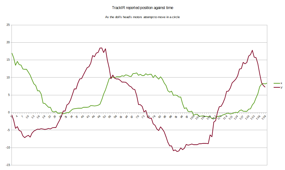
Unfortunately the movement of the head is extremely jerky. to quantify this, lets track the position accurately.
To do so, I mounted a TrackIR: 3 small reflective markers, which are then picked up by a camera. The position of the reflective markers are then determined, and the 6DOF position of the head calculated.
To actually log the data from TrackIR was tricky. To achieve this, I used FreePIE – an application for ‘bridging and emulating input devices’. It supports TrackIR as an input, and allows you to run a python function on input.
I wrote the following script to output CSV:
#Use Z to force flushing file to disk
import os
def update():
# Note that you need to set the
# curves for these to 1:1 in the TrackIR gui, which needs to be running
# at the same time.
yaw = trackIR.yaw
pitch = trackIR.pitch
roll = trackIR.roll
x = trackIR.x
y = trackIR.y
z = trackIR.z
csv_str = yaw.ToString() + "," + pitch.ToString() + "," + roll.ToString() + "," + x.ToString() + "," + y.ToString() + "," + z.ToString() + "\n"
#diagnostics.debug(csv_str)
f.write(csv_str)
if starting:
global f
trackIR.update += update
f = open("trackir output.csv","w")
diagnostics.debug("Logging to: " + os.path.realpath(f.name))
f.write("yaw,pitch,roll,x,y,z\n")
if keyboard.getPressed(Key.Z):
f.flush()
diagnostics.debug("flushing")
And taped the head tracker like so:
Note 1: I also set the TrackIR response curves to all be 1:1 and disabled smoothing of the input. We want the raw data. Although I later realised that freepie exposes the raw data, so I could have just used that instead.
Note 2: If you enable logging in FreePIE, it outputs the log to “C:\Program Files (x86)\FreePIE\trackirworker.txt”
Note 3: For some reason, FreePIE is only updating the TrackIR readings at 4hz. I don’t know why – I looked into the code, but without much success. I filed a bug.
And here are the results:
There is a lot of a jerkiness here. This is supposed to look like a beautiful sinusoidal curve:
To fix this, and make the movement smooth, we need to understand where this jerkiness comes from.
Source of jerkiness
A quick word about motivation: For almost my entire life, I’ve wanted to build robots with smooth natural-looking movement, and I’ve hated the unnatural jerkiness that you often see.
A quick word about terminology: ‘Jerkiness’ has a real technical meaning – it is the function of position over time, differentiated 3 times. Since we are aiming for a circular movement, and since the 3rd order differential of a sinusoidal movement is still sinusoidal, even in the ideal situation there is still technically a non-zero jerk. So here I mean jerkiness in a more informal manor. I have previously written about, and written code for, motion planning with a guaranteed jerk of 0 when controlling a car, for which the jerkiness really must be minimized to prevent whiplash and discomfort.
We must understand how a servo works:
How a servo works
A servo is a small geared DC motor, a potentiometer to measure position, and a control circuit that presumably uses some basic PID algorithm to power the motor to try to match the potentiometer reading to the pulse width given on the input line:
To prevent the motor from ‘rocking’ back and forth around the desired value, the control circuit implements a ‘dead bandwith’ – a region in which it considers the current position to be ‘close enough’ to the given pulse.
For the MG996R servo that I’m using, the spec sheet says:
Note the ‘Dead band width’ of 5µs. The servo moves about 130 degrees when given a duty cycle between 800µs to 2200µs. NOTE: This means that the maximum duty cycle is only about 10% of the PWM period.
So this means that we move approximately 10µs per degree: (2200µs – 800µs)/130° ≈10µs.
So our dead band width is approximately 0.5°. Note that that means ±0.25°.
The arduino Servo::write(int angle) command takes an integer number of degrees, and by default is configured to 5µs per degree (2400µs – 544µs)/180° ≈10µs this means that we are introducing four times as much ‘jerkiness’ into our movement than we need to, simply from sloppy API usage. (Numbers taken from github Servo.h code)
So lets change the code to use the four times as accurate: Servo::writeMicroseconds(int microseconds) which lets us specify the number of microseconds for the duty cycle:
#include
Servo up_down_servo; // create servo object to control a servo
Servo left_right_servo; // create servo object to control a servo
int pos = 0; // variable to store the servo position
void servoAccurateWrite(const Servo &servo, float angle) {
/* 544 default used by Servo object, but ~800 on MG996R) */
const int min_duty_cycle_us = MIN_PULSE_WIDTH;
/* 2400 default used by Servo object, but ~2200 on MG996R) */
const int max_duty_cycle_us = MAX_PULSE_WIDTH;
/* Default used by Servo object, but ~130 on MG996R */
const int min_to_max_angle = 180;
const int duty_cycle_us = min + angle * (max - min)/min_to_max_angle;
servo.writeMicroseconds(duty_cycle_us);
}
void setup() {
up_down_servo.attach(8); // attaches the servo on pin 8 to the servo object
up_down_servo.write(170); // Maximum is 170 and that's looking forward, and smallest is about 140 and that is looking a bit downwards
left_right_servo.attach(9); // attaches the servo on pin 9 to the servo object
left_right_servo.write(170); // 155 is facing forward. 170 is looking to the left for him
Serial.begin(115200);
Serial.println("up_down, left_right"); // Output a CSV stream, showing the desired positions
}
void loop() {
const float graduations = 1000.0;
for (pos = 0; pos < graduations; pos++) {
const float up_down_angle = 160+10*sin(pos / graduations * 2.0 * 3.1415);
const float left_right_angle = 155+5*cos(pos / graduations * 2.0 * 3.1415);
servoAccurateWrite(left_right_servo, left_right_angle);
servoAccurateWrite(up_down_servo, up_down_angle);
Serial.print(up_down_angle);
Serial.print(",");
Serial.println(left_right_angle);
delay(15);
}
}
And the result of the position, as reported by TrackIR:
What a huge difference this makes! This is much more smooth. It doesn’t look very sinusoidal, but it’s a lot smoother.
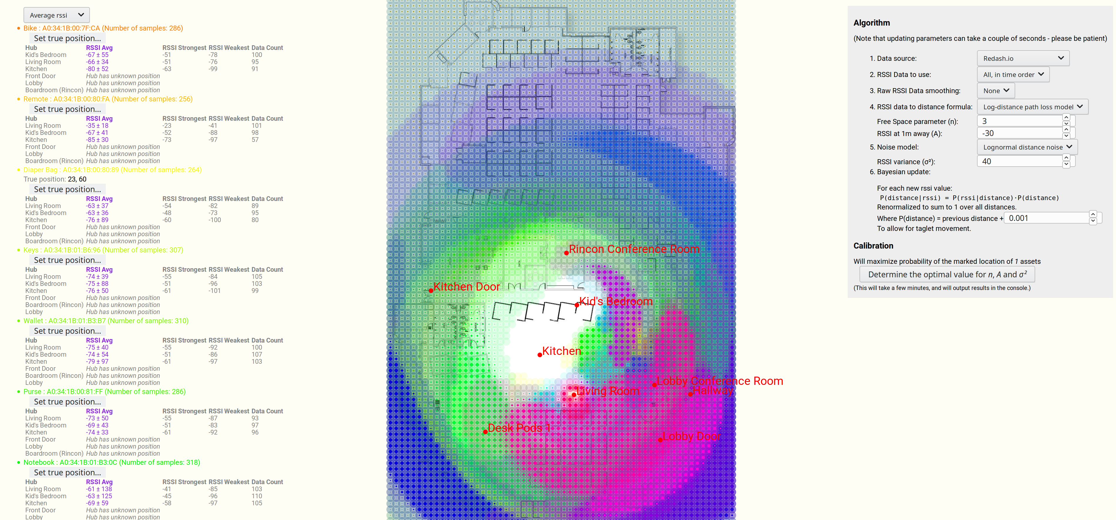
Imagine you have a bluetooth device somewhere in your house, and you want to try to locate it. You have several other devices in the house that can see it, and so you want to triangulate its position.
This article is about the result I achieved, and the methodology.
I spent two solid weeks working on this, and this was the result:
Estimating the most probable position of a bluetooth device, based on 7 strength readings.
We are seeing a map, overlaid in blue by the most likely position of a lost bluetooth device.
And a more advanced example, this time with many different devices, and a more advanced algorithm (discussed further below).
Note that some of the devices have very large uncertainties in their position.
Estimating position of multiple bluetooth devices, based on RSSI strength.
There are quite a few articles, video and books on estimating the distance of a bluetooth device (or wifi hub) based on knowing the RSSI signal strength readings.
But I couldn’t find any that gave the uncertainty of that estimation.
Noise is Normally distributed, with mean 0 and variance σ²
d is our distance (above) or estimated distance (below)
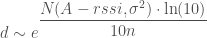
Rearranging to get an estimated distance, we get:
Now Noise is sampled from a Normal distribution, with mean = 0 and variance = σ², so let’s write our estimated d as a random variable:
Important note: Note that random variable d is distributed as the probability of the rssi given the distance. Not the probability of the distance given the rssi. This is important, and it means that we need to at least renormalize the probabilities over all possible distances to make sure that they add up to 1. See section at end for more details.
Adding a constant to a normal distribution just shifts the mean:
Now let’s have a bit of fun, by switching it to base e. This isn’t actually necessary, but it makes it straightforward to match up with wikipedia’s formulas later, so:
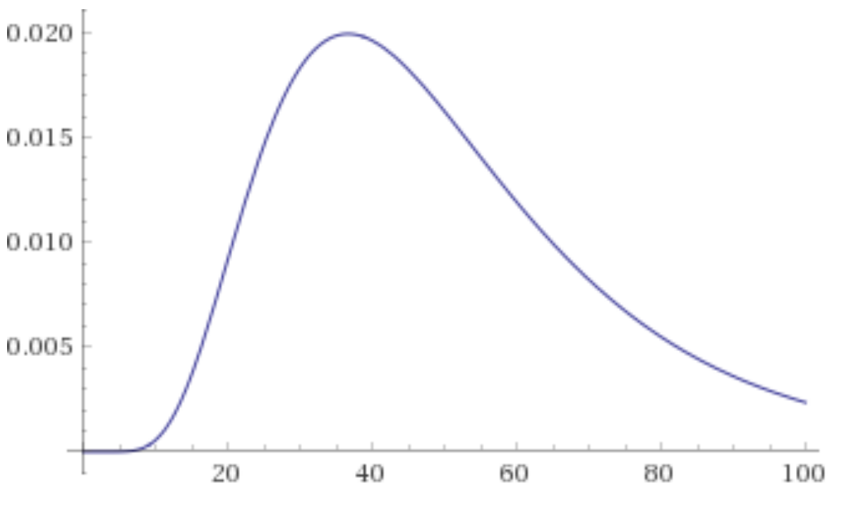
Distance in meters against probability density, for an rssi value of -80, A=-30, n=3, sigma^2=40
Bayes Theorem
I mentioned earlier:
Important note: Note that random variable d is distributed as the probability of the rssi given the distance. Not the probability of the distance given the rssi. This is important, and it means that we need to at least renormalize the probabilities over all possible distances to make sure that they add up to 1. See section at end for more details.
So using the above graph as an example, say that our measured RSSI was -80 and the probability density for d = 40 meters is 2%.


 is a
is a