Samurai Robot: Part 1

December 28, 2019November 8, 2021 / John Tapsell / 1 Comment

Samurai Robot Series:

I saw this for sale in a Christmas market for 500 yen (~$5 USD) and immediately bought it. My friends questioned my sanity, since it’s for “boy’s day” (It’s a “五月人形”) and we have no boys.

But, I could see the robotic potential!

Note: I have put the gold plated metal through an ultrasonic cleaner and buffed them with British Museum wax. But I’m not sure how to remove the corrosion – please message me if you have any ideas.

Next step is to build a wooden skeleton to mount the motors:

Ul0dLoX

I’ve used 2 MG996 servo motors (presumably clones).

And a quick and dirty arduino program to move the head in a circular motion:


#include 

Servo up_down_servo;     // create servo object to control a servo
Servo left_right_servo;  // create servo object to control a servo

int pos = 0;    // variable to store the servo position

void setup() {
  up_down_servo.attach(8);  // attaches the servo on pin 8 to the servo object
  up_down_servo.write(170); // Maximum is 170 and that's looking forward, and smallest is about 140 and that is looking a bit downwards

  left_right_servo.attach(9);  // attaches the servo on pin 9 to the servo object
  left_right_servo.write(170); // 155 is facing forward.  170 is looking to the left for him
  Serial.begin(115200);
  Serial.println("up_down, left_right");  // Output a CSV stream, showing the desired positions
}

void loop() {
  const float graduations = 1000.0;

  for (pos = 0; pos &lt; graduations; pos++) {
    const float up_down_angle = 160+10*sin(pos / graduations * 2.0 * 3.1415);
    const float left_right_angle = 155+5*cos(pos / graduations * 2.0 * 3.1415);
    left_right_servo.write(left_right_angle);
    up_down_servo.write(up_down_angle);
    Serial.print(up_down_angle);
    Serial.print(",");
    Serial.println(left_right_angle);
    delay(15);
  }
}

And the result:


Jerky Movement
Unfortunately the movement of the head is extremely jerky.  to quantify this, lets track the position accurately.
To do so, I mounted a TrackIR:  3 small reflective markers, which are then picked up by a camera.  The position of the reflective markers are then determined, and the 6DOF position of the head calculated.
To actually log the data from TrackIR was tricky.  To achieve this, I used FreePIE – an application for ‘bridging and emulating input devices’.   It supports TrackIR as an input, and allows you to run a python function on input.
I wrote the following script to output CSV:
#Use Z to force flushing file to disk
import os
def update():
    # Note that you need to set the
    # curves for these to 1:1 in the TrackIR gui, which needs to be running
    # at the same time.
 &nbsp;&nbsp; yaw = trackIR.yaw
 &nbsp;&nbsp; pitch = trackIR.pitch
 &nbsp;&nbsp; roll = trackIR.roll
&nbsp;&nbsp;&nbsp; x = trackIR.x
 &nbsp;&nbsp; y = trackIR.y
 &nbsp;&nbsp; z = trackIR.z
 &nbsp;&nbsp; csv_str = yaw.ToString() + "," + pitch.ToString() + "," + roll.ToString() +&nbsp;&nbsp;"," + x.ToString()&nbsp;&nbsp;+ "," + y.ToString()&nbsp;&nbsp;+ "," + z.ToString() + "\n"
&nbsp;&nbsp;&nbsp; #diagnostics.debug(csv_str)
&nbsp;&nbsp;&nbsp; f.write(csv_str)
if starting:
 &nbsp;&nbsp; global f
&nbsp;&nbsp;&nbsp; trackIR.update += update
&nbsp;&nbsp;&nbsp; f = open("trackir output.csv","w")
&nbsp;&nbsp;&nbsp; diagnostics.debug("Logging to:&nbsp;&nbsp;" + os.path.realpath(f.name))
&nbsp;&nbsp;&nbsp; f.write("yaw,pitch,roll,x,y,z\n")
if keyboard.getPressed(Key.Z):
&nbsp;&nbsp;&nbsp; f.flush()
&nbsp;&nbsp;&nbsp; diagnostics.debug("flushing")

And taped the head tracker like so:

Note 1: I also set the TrackIR response curves to all be 1:1 and disabled smoothing of the input. We want the raw data. Although I later realised that freepie exposes the raw data, so I could have just used that instead.
Note 2: If you enable logging in FreePIE, it outputs the log to “C:\Program Files (x86)\FreePIE\trackirworker.txt”
Note 3: For some reason, FreePIE is only updating the TrackIR readings at 4hz. I don’t know why – I looked into the code, but without much success. I filed a bug.
And here are the results:

There is a lot of a jerkiness here.  This is supposed to look like a beautiful sinusoidal curve: 
To fix this, and make the movement smooth, we need to understand where this jerkiness comes from.
Source of jerkiness
A quick word about motivation:  For almost my entire life, I’ve wanted to build robots with smooth natural-looking movement, and I’ve hated the unnatural jerkiness that you often see.
A quick word about terminology:  ‘Jerkiness’ has a real technical meaning – it is the function of position over time, differentiated 3 times.  Since we are aiming for a circular movement, and since the 3rd order differential of a sinusoidal movement is still sinusoidal, even in the ideal situation there is still technically a non-zero jerk.  So here I mean jerkiness in a more informal manor.  I have previously written about, and written code for, motion planning with a guaranteed jerk of 0 when controlling a car, for which the jerkiness really must be minimized to prevent whiplash and discomfort.
We must understand how a servo works:
How a servo works
A servo is a small geared DC motor, a potentiometer to measure position, and a control circuit that presumably uses some basic PID algorithm to power the motor to try to match the potentiometer reading to the pulse width given on the input line:
         
 
         
 
  
  
To prevent the motor from ‘rocking’ back and forth around the desired value, the control circuit implements a ‘dead bandwith’ – a region in which it considers the current position to be ‘close enough’ to the given pulse.
For the MG996R servo that I’m using, the spec sheet says:

Note the ‘Dead band width’ of 5µs.  The servo moves about 130 degrees when given a duty cycle between 800µs to 2200µs.  NOTE:  This means that the maximum duty cycle is only about 10% of the PWM period.
So this means that we move approximately 10µs per degree: (2200µs – 800µs)/130° ≈ 10µs.
So our dead band width is approximately 0.5°.  Note that that means ±0.25°.
The arduino Servo::write(int angle) command takes an integer number of degrees, and by default is configured to 5µs per degree (2400µs – 544µs)/180° ≈ 10µs this means that we are introducing four times as much ‘jerkiness’ into our movement than we need to, simply from sloppy API usage.  (Numbers taken from github Servo.h code)
So lets change the code to use the four times as accurate:  Servo::writeMicroseconds(int microseconds)  which lets us specify the number of microseconds for the duty cycle:
#include 

Servo up_down_servo;     // create servo object to control a servo
Servo left_right_servo;  // create servo object to control a servo

int pos = 0;    // variable to store the servo position

void servoAccurateWrite(const Servo &amp;servo, float angle) {
  /* 544 default used by Servo object, but ~800 on MG996R) */
  const int min_duty_cycle_us = MIN_PULSE_WIDTH;
  /* 2400 default used by Servo object, but ~2200 on MG996R) */
  const int max_duty_cycle_us = MAX_PULSE_WIDTH;
  /* Default used by Servo object, but ~130 on MG996R */
  const int min_to_max_angle = 180;
  const int duty_cycle_us = min + angle * (max - min)/min_to_max_angle;
  servo.writeMicroseconds(duty_cycle_us);
}

void setup() {
  up_down_servo.attach(8);  // attaches the servo on pin 8 to the servo object
  up_down_servo.write(170); // Maximum is 170 and that's looking forward, and smallest is about 140 and that is looking a bit downwards

  left_right_servo.attach(9);  // attaches the servo on pin 9 to the servo object
  left_right_servo.write(170); // 155 is facing forward.  170 is looking to the left for him
  Serial.begin(115200);
  Serial.println("up_down, left_right");  // Output a CSV stream, showing the desired positions
}

void loop() {
  const float graduations = 1000.0;

  for (pos = 0; pos &lt; graduations; pos++) {
    const float up_down_angle = 160+10*sin(pos / graduations * 2.0 * 3.1415);
    const float left_right_angle = 155+5*cos(pos / graduations * 2.0 * 3.1415);
    servoAccurateWrite(left_right_servo, left_right_angle);
    servoAccurateWrite(up_down_servo, up_down_angle);
    Serial.print(up_down_angle);
    Serial.print(",");
    Serial.println(left_right_angle);
    delay(15);
  }
}

And the result of the position, as reported by TrackIR:

What a huge difference this makes! This is much more smooth. It doesn’t look very sinusoidal, but it’s a lot smoother.

Wifi / bluetooth RSSI signal strength to distance

December 28, 2019December 28, 2019 / John Tapsell / 1 Comment

Imagine you have a bluetooth device somewhere in your house, and you want to try to locate it. You have several other devices in the house that can see it, and so you want to triangulate its position.

This article is about the result I achieved, and the methodology.

I spent two solid weeks working on this, and this was the result:

RSSI Location of a single bluetooth device

Estimating the most probable position of a bluetooth device, based on 7 strength readings.

We are seeing a map, overlaid in blue by the most likely position of a lost bluetooth device.

And a more advanced example, this time with many different devices, and a more advanced algorithm (discussed further below).

Note that some of the devices have very large uncertainties in their position.

Estimating position of multiple bluetooth devices, based on RSSI strength.

And to tie it all together, a mobile app:

Find It App Screen

Methodology

There are quite a few articles, video and books on estimating the distance of a bluetooth device (or wifi hub) based on knowing the RSSI signal strength readings.

But I couldn’t find any that gave the uncertainty of that estimation.

So here I derive it myself, using the Log-distance_path loss model

$rssi = -10n \log_{10}(d) + A + Noise$

In this model:

rssi is the signal strength, measured in dB
n is a ‘path loss exponent’:
A is the rssi value at 1 meter away
Noise is Normally distributed, with mean 0 and variance σ²
d is our distance (above) or estimated distance (below)

Rearranging to get an estimated distance, we get:

$d = 10^{\dfrac{A - rssi + Noise}{10n}}$

Now Noise is sampled from a Normal distribution, with mean = 0 and variance = σ², so let’s write our estimated d as a random variable:

$d \sim 10^{\dfrac{A - rssi + N(0,\sigma^2)}{10n}}$

Important note: Note that random variable d is distributed as the probability of the rssi given the distance. Not the probability of the distance given the rssi. This is important, and it means that we need to at least renormalize the probabilities over all possible distances to make sure that they add up to 1. See section at end for more details.

Adding a constant to a normal distribution just shifts the mean:

$d \sim 10^{\dfrac{N(A - rssi,\sigma^2)}{10n}}$

Now let’s have a bit of fun, by switching it to base e. This isn’t actually necessary, but it makes it straightforward to match up with wikipedia’s formulas later, so:

$d \sim e^{\dfrac{N(A - rssi,\sigma^2) \cdot \ln(10)}{10n}}$

$d \sim e^{N(A - rssi,\sigma^2)\cdot \ln(10)/10n}$

Where $e^{N(A - rssi,\sigma^2)}$ is a Lognormal distribution:

$d \sim \mathrm{Lognormal}(A - rssi,\sigma^2)^{\frac{\ln(10)}{10n}}$

We can now use the rule in https://en.wikipedia.org/wiki/Log-normal_distribution that:

And we thus get our final result:

$\boxed{d \sim \mathrm{Lognormal}((A - rssi)\cdot\ln(10)/(10n),\sigma^2\cdot\ln(10)^2/(10n)^2)}$

Example plot: Plot[PDF[LogNormalDistribution[(-30 – (-80))*log(10)/(10*3),sqrt(40)*log(10)/(10*3)],x],{x,0,100}]

Distance in meters against probability density, for an rssi value of -80, A=-30, n=3, sigma^2=40

Bayes Theorem

I mentioned earlier:

Important note: Note that random variable d is distributed as the probability of the rssi given the distance. Not the probability of the distance given the rssi. This is important, and it means that we need to at least renormalize the probabilities over all possible distances to make sure that they add up to 1. See section at end for more details.

So using the above graph as an example, say that our measured RSSI was -80 and the probability density for d = 40 meters is 2%.

This means:

P(measured_rssi = -80|distance=40m) = 2%

But we actually want to know is:

P(distance=40m | measured_rssi=-80)

So we need to apply Bayes theorem:

So we have an update rule of:

P(distance=40m | measured_rssi=-80) = P(measured_rssi = -80|distance=40m) * P(distance=40m)

Where we initially say that all distances within an area are equally likely = P(distance=40m) = 1/area

And we renormalize the probability to ensure that sum of probabilities over all distances = 1.

Laplace Transform – visualized

February 12, 2019May 30, 2023 / John Tapsell / 2 Comments

The Laplace Transform is a particular tool that is used in mathematics, science, engineering and so on. There are many books, web pages, and so on about it.

My animations are now on Wikipedia: https://en.wikipedia.org/wiki/Laplace_transform

And yet I cannot find a single decent visualization of it! Not a single person that I can find appears to have tried to actually visualize what it is doing. There are plenty of animations for the Fourier Transform like:

fourier

But nothing for Laplace Transform that I can find.

So, I will attempt to fill that gap.

What is the Laplace Transform?

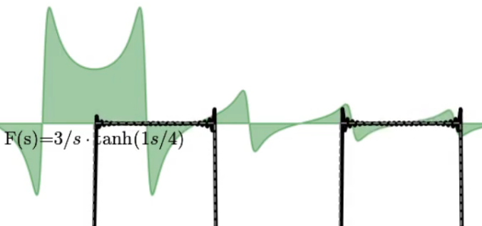
It’s a way to represent a function that is 0 for time < 0 (typically) as a sum of many waves that look more like:

Graph of $e^t cos(10t)$

Note that what I just said isn’t entirely true, because there’s an imaginary component here too, and we’re actually integrating. So take this as a crude idea just to get started, and let’s move onto the math to get a better idea:

Math

The goal of this is to visualize how the Laplace Transform works:

$\displaystyle\mathscr{L}\{f(t)\}=F(s)$

To do this, we need to look at the definition of the inverse Laplace Transform: (Using Mellin’s inverse formula: https://en.wikipedia.org/wiki/Inverse_Laplace_transform )

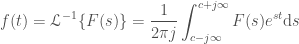
$\displaystyle f(t) = \mathscr{L}^{-1}\{F(s)\}=\frac{1}{2\pi j}\int^{c+j\infty}_{c-j\infty} F(s)e^{st}\mathrm{d}s$

While pretty, it’s not so nice to work with, so let’s make the substitution:

$\displaystyle s := c+jr$

so that our new limits are just $\infty$ to $-\infty$ , and $\mathrm{d}s/\mathrm{d}r = j$ giving:

$\displaystyle f(t) = \mathscr{L}^{-1}\{F(s)\}=\frac{1}{2\pi j}\int^{\infty}_{-\infty} F(c+jr)e^{(c+jr)t}j\mathrm{d}r$

$\displaystyle = \frac{1}{2\pi}\int^{\infty}_{-\infty} F(c+jr)e^{(c+jr)t}\mathrm{d}r$

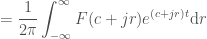
Which we will now approximate as:

$\displaystyle \approx \frac{1}{2\pi}\sum^{n}_{i=-n} F(c+jr_i)e^{(c+jr_i)t}\Delta r_i$

Code

The code turned out to be a bit too large for a blog post, so I’ve put it here:

https://github.com/johnflux/laplace-transform-visualized/blob/master/Laplace%20Transform.ipynb

Results

Note: The graphs say “Next frequency to add: … where $s = c+rj$ “, but really it should be “Next two frequencies to add: … where $s = c\pm rj$ ” since we are adding two frequencies at a time, in such a way that their imaginary parts cancel out, allowing us to keep everything real in the plots. I fixed this comment in the code, but didn’t want to rerender all the videos.

A cubic polynomial:

A cosine wave:

Now a square wave. This has infinities going to infinity, so it’s not technically possible to plot. But I tried anyway, and it seems to visually work:

Note the overshoot ‘ringing’ at the corners in the square wave. This is the Gibbs phenomenon and occurs in Fourier Transforms as well. See that link for more information.

Now some that it absolutely can’t handle, like: $\delta(t)$ . (A function that is 0 everywhere, except a sharp peak at exactly time = 0). In the S domain, this is a constant, meaning that we never converge. But visually it’s still cool.

Note that this never ‘settles down’ (converges) because the frequency is constantly increasing while the magnitude remains constant.

There is visual ‘aliasing’ (like how a wheel can appear to go backwards as its speed increases). This is not “real” – it is an artifact of trying to render high frequency waves. If we rendered (and played back) the video at a higher resolution, the effect would disappear.

At the very end, it appears as if the wave is just about to converge. This is not a coincidence and it isn’t real. It happens because the frequency of the waves becomes too high so that we just don’t see them, making the line appear to go smooth, when in reality the waves are just too close together to see.

The code is automatically calculating this point and setting our time step such that it only breaksdown at the very end of the video. If make the timestep smaller, this effect would disappear.

And a simple step function:

A sawtooth:

Compiler is ignoring my C code!

February 8, 2019February 8, 2019 / John Tapsell / Leave a comment

Sometimes you come across a weird bug where the output seems to be completely impossible. And it’s extremely hard to debug or search on google for, if you don’t know about this:

If your code has Undefined Behaviour, the compiler is allowed to assume it won’t happen, and can ‘optimize out’ chunks of your code.

Here’s a code snippet in a real bug I found yesterday:

#define FOO_SIZE 10
int foo2[FOO_SIZE];
...
int n=0;
do {
    p->foo[n] = foo2[n];
    n++;
} while( (foo2[n] != 0) && (n < FOO_SIZE) );
printk("n is %d\n", n);

This printed out:

   n is 165

and the system crashed.

But how can n become larger than FOO_SIZE=10 ? Because the compiler ‘optimized’ away the check. Here’s the asm:

} while( (foo2[n] != 0) && (n < FOO_SIZE) );
   21a14:       f813 2f01       ldrb.w  r2, [r3, #1]!
   21a18:       2a00            cmp     r2, #0
   21a1a:       d1f8            bne.n   21a0e <NV_Get+0x82>
   21a1c:       e7ca            b.n     219b4 <NV_Get+0x28>

What we are seeing here is that the “n < FOO_SIZE” check has been completely removed by the compiler. Why?

Because in the check, if n == FOO_SIZE, we would be checking if: foo2[FOO_SIZE] != 0. But this is out of bounds for foo. The compiler knows that this is out of bounds, and so knows that this is undefined behaviour. But the compiler is allowed to assume that undefined behaviour doesn’t happen, and so it assumes that n can NEVER be >= FOO_SIZE. Thus it can remove the n < FOO_SIZE check.

This can be fixed by switching the order of the && like:

} while( (n < FOO_SIZE) && (foo2[n] != 0) );

Or, by checking n-1 instead (which is slightly different behaviour, but good enough for me. I was changing a lot of code with this bug.)

} while( (foo2[n-1] != 0) && (n < FOO_SIZE) );
   21a26:       7809            ldrb    r1, [r1, #0]
   21a28:       2900            cmp     r1, #0
   21a2a:       d0c3            beq.n   219b4 <NV_Get+0x28>
   21a2c:       429a            cmp     r2, r3
   21a2e:       d1f5            bne.n   21a1c <NV_Get+0x90>
   21a30:       e7c0            b.n     219b4 <NV_Get+0x28>

Now we see the second comparison in the asm.

Calibrating Cameras

May 17, 2018May 23, 2018 / John Tapsell / Leave a comment

It is common to want to calibrate cameras for lens distortion.

First print out a standard chequerboard image, and take some photos of it from various angles. You can print out images, for example, here:

https://calib.io/pages/camera-calibration-pattern-generator

Here I assume these photos are in camera_cal/calibration*.jpg

Even if you ultimately want to calibrate the images from c++, python, javascript etc, the calibration itself can be done separately, in a more convenient language, producing a matrix that you can use pretty much anywhere. In my case, I calibrate in a jypter notebook, but use the matrix in c++.

%matplotlib inline

import numpy as np
import cv2
import glob
import matplotlib.pyplot as plt
#%matplotlib qt

# prepare object points, like (0,0,0), (1,0,0), (2,0,0) ....,(6,5,0)
objp = np.zeros((6*9,3), np.float32)
objp[:,:2] = np.mgrid[0:9,0:6].T.reshape(-1,2)

# Arrays to store object points and image points from all the images.
objpoints = [] # 3d points in real world space
imgpoints = [] # 2d points in image plane.

# Make a list of calibration images
images = glob.glob('camera_cal/calibration*.jpg')

# Step through the list and search for chessboard corners
for fname in images:
img = cv2.imread(fname)
gray = cv2.cvtColor(img,cv2.COLOR_BGR2GRAY)

# Find the chessboard corners
ret, corners = cv2.findChessboardCorners(gray, (9,6),None)

# If found, add object points, image points
if ret == True:
objpoints.append(objp)
imgpoints.append(corners)

# Draw and display the corners
img = cv2.drawChessboardCorners(img, (9,6), corners, ret)
plt.imshow(img)
plt.show()

ret, camera_undistort_matrix, camera_undistort_dist, rvecs, tvecs = cv2.calibrateCamera(objpoints, imgpoints, gray.shape[::-1], None, None)

fname = images[8]
img = cv2.imread(fname)
gray = cv2.cvtColor(img,cv2.COLOR_BGR2GRAY)
ret, corners = cv2.findChessboardCorners(gray, (9,6),None)
print(ret)
img = cv2.drawChessboardCorners(img, (9,6), corners, ret)
dst = cv2.undistort(img, camera_undistort_matrix, camera_undistort_dist, None, camera_undistort_matrix)
img = np.concatenate((img, dst), axis=1)
plt.imshow(img)
cv2.imwrite("output_images/undistort_chessboard.png", img)
plt.show()

output_2_1

On the left is the original photo, and on the right is after applying the undistortion matrix warp.

import pickle
with open('camera_undistort_matrix.pkl', 'wb') as f:
pickle.dump((camera_undistort_matrix, camera_undistort_dist), f)
print(camera_undistort_matrix)

[[ 1.15777829e+03 0.00000000e+00 6.67113865e+02]
[ 0.00000000e+00 1.15282230e+03 3.86124659e+02]
[ 0.00000000e+00 0.00000000e+00 1.00000000e+00]]

img = cv2.imread("test_images/straight_lines1.jpg")
dst = cv2.undistort(img, camera_undistort_matrix, dist, None, camera_undistort_matrix)
img = np.concatenate((img,dst),axis=1)
img_rgb = cv2.cvtColor(np.asarray(img), cv2.COLOR_BGR2RGB)
plt.imshow(img_rgb)
cv2.imwrite("output_images/undistort_straight_lines1.png", img)
plt.show()

In the top left is the original image, in the top right is the undistorted image. There is little difference to the eye, but the distortion lets us to now apply further distortions such as a perspective transform to provide an apparent “top-down view”.

It is also useful for applying other transforms key to stitching together images from multiple cameras.

Pictures of my 360 Camera Software

March 8, 2018March 9, 2018 / John Tapsell / Leave a comment

This is something that I’ve been working on for over 2 years now.

I’ve mentioned it before, but I thought I’d add some photos.

And we have the cameras hooked up to cool ‘robots’ / gantry systems:

Machine Translated renaming of files

February 22, 2018February 23, 2018 / John Tapsell / Leave a comment

I needed to rename a whole load of files that were in Japanese. So I wrote a python program that translates the filename using google translate.

It’s not at all fancy, just run it and pass the filenames to translate and rename.

E.g.:

$ ls
こんにちは世界.png
$ sudo pip3 install googletrans
$ translate_rename.py こんにちは世界.png
こんにちは世界.png -> Hello_World.png
$ ls
Hello_World.png

#!/usr/bin/python3

import sys, re, os
from googletrans import Translator

translator = Translator()

sourceLanguage = 'ja'
destLanguage = 'en'

# Set to false to actually rename the files
dryRun = True

def translate_and_rename(filename):
    filenameSplit = filename.rsplit('.',1)
    translated = translator.translate(filenameSplit[0], src=sourceLanguage, dest=destLanguage).text
    translated = re.sub( '[^a-zA-Z0-9.]+', '_', translated).strip().title()
    if len(filenameSplit) > 1:
        translated += '.' + filenameSplit[1]
    if filename == translated:
        print(filename, ' (unchanged)')
    else:
        print(filename, " -> ", translated)
        if not dryRun:
            os.rename(filename, translated)

def main(argv):
    if len(argv) == 1:
        print("Need to pass filenames to translate and rename")

    for x in argv[1:]:
        translate_and_rename(x)
    if dryRun:
        print()
        print("  Dry run only - no actual changes made  ")
        print()
        print("Edit this file and set DryRun to True")

if __name__ == "__main__":
    main(sys.argv)

TypeScript + lodash map and filter

December 8, 2017January 11, 2018 / John Tapsell / Leave a comment

I love TypeScript. I use it whenever I can. That said, sometimes it can be… interesting. Today, out of the blue, I got the typescript error in code that used to work:

[06:53:30]  typescript: src/mycode.ts, line: 57 
            Property 'video' does not exist on type 'number | (<U>(callbackfn: (value: Page, index: number, 
            array: Page[]) => U, thisA...'. Property 'video' does not exist on type 'number'.

The code looks like:

return _.chain(pages)
        .filter((s, sIdx) => s.video || s.videoEmbedded)
        .map((s, sIdx) => {
            if (s.video) { ... }

Can you spot the ‘error’?

The problem is that s.video || s.videoEmbedded isn’t returning a boolean. It’s return a truthy value, but not a boolean. And the lodash typescript developers made a change 1 month ago that meant that filter() would only accept booleans, not any truthy value. And the lodash typescript developers are finding that fixing this becomes very complicated and complex. See the full conversation here:

https://github.com/DefinitelyTyped/DefinitelyTyped/issues/21485

(Open issue at time of writing. Please leave me feedback or message me if you see this bug get resolved)

The workaround/fix is to just make sure it’s a boolean. E.g. use !! or Boolean(..) or:

return _.chain(pages)
        .filter((s, sIdx) => s.video !== null || s.videoEmbedded !== null )
        .map((s, sIdx) => {
            if (s.video) { ... }

I don’t like PID control

September 14, 2017September 15, 2017 / John Tapsell / 1 Comment

I’ve implemented PID control far too many times now, and I’ve never been that happy with the results.

It is simple to implement, but tricky to tune. My thick control theory book says that 95% of commercial in-use PID systems are sub-optimally tuned. And I can believe it.

I’ve been recently playing with other systems, and currently I really like Model Predictive Control. It does require some significant compute power, which was a big problem when it was invented, but not so much any more. (As a side point, I’d like to implement MPC in tensorflow. That would be cool, and could probably be done in a weekend).

I wrote a PID control system for a self driving car. It is dumbly auto-tuned, so to speak, by a simple twiddle method. It tests out a particular set of PID values for one minute, resets the track, then picks a new set of PID values based on the best seen values, changed slightly.

The results are… very underwhelming.

The same driving but using Model Predictive Control, below, starts to look a lot nicer. For reference, the PID control took a total of two days to implement, and the MPC took a total of three days. The MPC version also has an additional complication – there’s a simulated delay of 100ms.

But I’m very pleased with the results. It’s a bit jerky here due to random latency variations, made worse by the screen recording software. I’ve got some ideas on trying to solve that by timestamping, but I don’t think I’ll have time to work on it.

I would love to try applying this MPC system to a Quadcopter. I’ve written quite a bit previously about latency problems with PID in a quadcopter: (In this video, the ufo-shaped quadcopter is attempting to move to, and maintain, a fixed position above the chair. Ignore the blue man 🙂 )

Why Kalman Filters are broken, and how to fix

July 23, 2017August 1, 2017 / John Tapsell / Leave a comment

Okay, so clickbait title, because I’m referring to the most common case of using a single Gaussian distribution to represent the current estimated position (for example) and for the measurement.

Here’s my problem with that:

They don’t take into account that sometimes things go wrong.

Now you may say ‘duh’, but it can cause some really serious problems if something does go wrong.

Say you have a self driving car. And the following happens:

Prior: You currently estimate the position of a person in front of you to be at position: x = 2m ± 0.5m aka X ~ N(2,0.5)
Data: Your instruments return a new measure: the person is now measured to be at position: x = 10m ± 0.5m aka X ~ N(10,0.5)
Posterior: You apply your Kalman Filter and it concludes that the position of the person is now at: x = 6m ± 0.25m aka X ~ N(6,0.25)

gaussian1

You are now extremely confident that the person is at x=6m despite you previously thinking that they were at a x=2m and your measurement data says that they are at x=10m. You, the self driving car, now happily drive at x=10m.

How confident would you, as a, human, really be that the person is at x=6m? Barely at all, right? So something has gone wrong here.

Here’s an example in a simulator. A car is driving from right to left and we are trying to track its true position with a Extended Kalman Filter. ◯ The red circles indicate data from the simulated LASER, ◔ blue circle circles are RADAR, and ▲ green triangles are the position estimated by a Kalman filter. At the bottom of the arc, a single bad LASER data point is injected.

Credit to Udacity for the simulator.

The result is that the predicted position goes way off, and takes many times steps to recover.

The blame all lies on Sherlock Holmes:

sherlock

The product of N(2,0.5) * N(10,0.5) results in a ridiculous improbable scenerio – we have to scale up the result by $10^{14}$ . i.e. treating the highly improbable as truth. Perhaps what Sherlock should have said is that it is far more likely that you were simply mistaken in elimination! i.e. your prior or data was wrong!

Fixing the basic Kalman Filter

Here’s a small change we could make. We can add a small probability of ‘wtf’ to our system.

Prior: You currently estimate the position of a person in front of you to be at position: $x_{prior} = 2 \pm 0.5$ plus a $W_{prior}$ chance of ‘wtf’: aka: $X \sim (1-W_{prior}) \cdot N(2,0.5) + W_{prior} \cdot \textrm{WTF}$
Data: Your instruments return a new measure: the person is now measured to be at position: $x_{data} = 10 \pm 0.5$ plus a $W_{data}$ chance of ‘wtf’: aka:
$X \sim (1-W_{data}) \cdot N(10,0.5) + W_{data} \cdot \textrm{WTF}$
Posterior: You apply your bayes rule. What do we get now? We need the product of these two random variables, and then normalize, by setting C such that the total integral is 1. $\displaystyle{ \left( (1-W_{prior}) \cdot N(2,0.5) + W_{prior} \cdot \textrm{WTF} \right) \cdot \left( (1-W_{data}) \cdot N(10,0.5) + W_{data} \cdot \textrm{WTF} \right) / C}$ (note that $N(10,0.5) \cdot N(2,0.5)$ is proportionate to a new Gaussian scaled by a factor $S$ ) $= ( (1-W_{prior}) \cdot (1-W_{data}) \cdot N(6,0.25) \cdot S + (1-W_{prior}) \cdot W_{data} \cdot N(2,0.5) +$
$W_{prior} \cdot (1-W_{data}) \cdot N(10,0.5) + W_{prior} \cdot W_{data} \cdot \textrm{WTF}^2 ) / C$ We know that the area must equal 1 for a PDF, so we can determine the scale factor C. See Appendix below for any technical details, including the formula for S and C.So we have a solution, but the solution is a gaussian mixture model – a sum of a gaussian for the combination, a gaussian for the prior, and a gaussian for the data. So let’s simply pick the one with the highest probability, and roll the other two into the WTF weight.

Here’s the result as an gif – the posterior is where the posterior would normally be, and the shaded blue area is our ‘wtf’ version of the posterior as a weighted mixture model:

Various different priors and data. There’s no updating step here – just showing different mean values for the prior and data. The posterior is kept centered to make it easier to see.

It looks pretty reasonable! If the prior and data agree to within their uncertainties, then the mixture model just returns the posterior. And when they disagree strongly, we return a mixture of them.

Let’s now make an approximation of that mixture model to a single gaussian, by choosing a gaussian that minimizes the KL divergence.

Screenshot_20170726_015120

Which results in the red line ‘Mixture Model Approximated’:

Different priors and data, with the red line showing this new method’s output. As above, there’s no update step here – it’s not a time series.

Now this red line looks very reasonable! When the prior and data disagree with each other, we have a prediction that is wide and covers both of them. But when they agree with each other to within their uncertainties, we get a result that properly combines both and gives us a posterior result that is more certain than either – i.e. we are adding information.

In total, the code to just take a prior and data and return a posterior is this:
(Note: I’ve assumed there are no covariances – i.e. no correlation in the error terms)

# prior input
mu1 = 5
variance1 = 0.5
# data input
mu2 = 6
variance2 = 0.5
# This is what you would normally do, in a standard Kalman Filter:
variance3 = 1/(1/variance1 + 1/variance2)
mu3 = (mu1/variance1 + mu2/variance2)*variance3

#But instead we will do:
S = 1/(np.sqrt(2*np.pi*variance1*variance2/variance3)) * np.exp(-0.5 * (mu1 - mu2)**2 * variance3/(variance1*variance2))
Wprior = 0.01 # 1% chance our prior is wrong
Wdata = 0.01 # 1% chance our data is wrong
C = (1-Wprior) * (1-Wdata) * S + (1-Wprior) * Wdata + Wprior * (1-Wdata)
weights = [
Wprior * (1-Wdata) /C, # weight of prior
(1-Wprior) * Wdata /C, # weight of data
(1-Wprior) * (1-Wdata) * S/C ] #weight of posterior
mu4 = weights[0]*mu1 + weights[1]*mu2 + weights[2] * mu3
variance4 = weights[0]*(variance1 + (mu1 - mu4)**2) + \
weights[1]*(variance2 + (mu2 - mu4)**2) + \
weights[2]*(variance3 + (mu3 - mu4)**2)

So at mu3 and variance3 is the green curve in our graphs and is the usual approach, while mu4 and variance4 is my new approach and is a better estimation of posterior.

The full ipython notebook code for everything produced here, is in git, here:

https://github.com/johnflux/Improved-Kalman-Filter/blob/master/kalman.ipynb

Results: Testing out in Simulator

Unfortunately, in my simulator my kalman filter has a velocity component, which I don’t actually take into in my analysis yet. My math completely ignores any dependent variables. The problem is that when we increase the uncertainty of the position then we also need to increase the uncertainty of the velocity.

To salvage this, I used just a small part of the code:

<div>
<div>double Scale = 1/(sqrt(2*M_PI*variance1*variance2/variance3)) * exp(-0.5 * (mu1 – mu2)*(mu1 – mu2) * variance3/(variance1*variance2));</div>
<div>
<div>
<div>if (Scale < 0.00000000001)
return; /* Just completely ignore this data point */</div>
</div>
</div>
</div>

The result is this:

Screenshot_20170802_012822

Appendix:

Just some technical notes, for completeness.

We can set $WTF = 1/(2A)$ where it can be anywhere between A and -A. We can take A to be large or even take the limit to infinity.
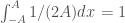It is a Probability Density Function since the area is 1: $\int^A_{-A} 1/(2A) dx = 1$ , and can set the Cauchy principal value of the integral to be 1 to keep it a PDF in the limit.
$\int^A_{-A} \textrm{WTF}^2(x) dx \to 0$ since: $\int^A_{-A} 1/(2A)^2 dx = 2A/(4A^2) = 1/(2A)$ which tends to 0 as $A \to \infty$ .
The scale factor S is simple but tedious to calculate:
The scale factor C can then be calculated by just setting the integral to equal 1 since it’s a PDF: $C = (1-W_{prior}) \cdot (1-W_{data}) \cdot S + (1-W_{prior}) \cdot W_{data} + W_{prior} \cdot (1-W_{data})$

	Bilal on Update: Release! ChatGPT clone…
	moon on Nokia 6110 Part 3 –…
	Lee V on Adobe After Effects
	John Tapsell on Nokia 6110 Part 3 –…
	Quackleb on Nokia 6110 Part 3 –…

John Tapsell

Director of Flux Programming Ltd – Available for hire! See 'About'!

Uncategorized