Ever wanted to export multiple layers in a Gimp or Photoshop image, with each layer as its own PNG, but the whole thing then wrapped up as an SVG?
The usefulness is that an artist can create an image of, say, a person, with eyes of various different colours in multiple layers. Then we can create an SVG file that we can embed in an html page, and then change the color of the eyes through Javascript.
So take this example. In this image we have a face made up of various layers, and the layers are further grouped in GroupLayers.

Combined layers

Layers in GroupLayers
So imagine having this image, then in Javascript on your page being able to swap out just the eye image. Or just the mouth image.
To achieve this, I had to modify an existing gimp python script from 5 years ago that has since bitrotted. Back when it was written, there was no such thing as group layers, so the script doesn’t work now. A bit of hacking, and I get:
#!/usr/bin/env python
# -*- coding: <utf-8> -*-
# Author: Erdem Guven <zuencap@yahoo.com>
# Copyright 2016 John Tapsell
# Copyright 2010 Erdem Guven
# Copyright 2009 Chris Mohler
# "Only Visible" and filename formatting introduced by mh
# License: GPL v3+
# Version 0.2
# GIMP plugin to export as SVG

# Save this to ~/.gimp-*/plug-ins/export_svg.py

from gimpfu import *
import os, re

gettext.install("gimp20-python", gimp.locale_directory, unicode=True)

def format_filename(imagename, layer):
	layername = layer.name.decode('utf-8')
	regex = re.compile("[^-\w]", re.UNICODE)
	filename = imagename + '-' + regex.sub('_', layername) + '.png'
	return filename

def export_layers(dupe, layers, imagename, path, only_visible, inkscape_layers):
	images = ""
	for layer in layers:
		if not only_visible or layer.visible:
			style=""
			if layer.opacity != 100.0:
				style="opacity:"+str(layer.opacity/100.0)+";"
			if not layer.visible:
				style+="display:none"
			if style != "":
				style = 'style="'+style+'"'

			if hasattr(layer,"layers"):
				image = '<g inkscape:groupmode="layer" inkscape:label="%s" %s>' % (layer.name.decode('utf-8'),style)
				image += export_layers(dupe, layer.layers, imagename, path, only_visible, inkscape_layers)
				image += '</g>'
				images = image + images
			else:
				filename = format_filename(imagename, layer)
				fullpath = os.path.join(path, filename);
				pdb.file_png_save_defaults(dupe, layer, fullpath, filename)

				image = ""
				if inkscape_layers:
					image = '<g inkscape:groupmode="layer" inkscape:label="%s" %s>' % (layer.name.decode('utf-8'),style)
					style = ""
				image += ('<image xlink:href="%s" x="%d" y="%d" width="%d" height="%d" %s/>\n' %
					(filename,layer.offsets[0],layer.offsets[1],layer.width,layer.height,style))
				if inkscape_layers:
					image += '</g>'
				images = image + images
		dupe.remove_layer(layer)
	return images

def export_as_svg(img, drw, imagename, path, only_visible=False, inkscape_layers=True):
	dupe = img.duplicate()

	images = export_layers(dupe, dupe.layers, imagename, path, only_visible, inkscape_layers)

	svgpath = os.path.join(path, imagename+".svg");
	svgfile = open(svgpath, "w")
	svgfile.write("""<?xml version="1.0" encoding="UTF-8" standalone="no"?>
<!-- Generator: GIMP export as svg plugin -->

<svg xmlns:xlink="http://www.w3.org/1999/xlink" """) 	if inkscape_layers: 		svgfile.write('xmlns:inkscape="http://www.inkscape.org/namespaces/inkscape" ') 	svgfile.write('width="%d" height="%d">' % (img.width, img.height));
	svgfile.write(images);
	svgfile.write("</svg>");

register(
	proc_name=("python-fu-export-as-svg"),
	blurb=("Export as SVG"),
	help=("Export an svg file and an individual PNG file per layer."),
	author=("Erdem Guven <zuencap@yahoo.com>"),
	copyright=("Erdem Guven"),
	date=("2016"),
	label=("Export as SVG"),
	imagetypes=("*"),
	params=[
		(PF_IMAGE, "img", "Image", None),
		(PF_DRAWABLE, "drw", "Drawable", None),
		(PF_STRING, "imagename", "File prefix for images", "img"),
		(PF_DIRNAME, "path", "Save PNGs here", os.getcwd()),
		(PF_BOOL, "only_visible", "Only Visible Layers?", False),
		(PF_BOOL, "inkscape_layers", "Create Inkscape Layers?", True),
		   ],
	results=[],
	function=(export_as_svg),
	menu=("<Image>/File"),
	domain=("gimp20-python", gimp.locale_directory)
	)

main()
(Note that if you get an error ‘cannot pickle GroupLayers’, this is a bug in gimp. It can be fixed by editing
350: gimpshelf.shelf[key] = defaults
)
Which when run, produces:
girl-Layer12.png
girl-Layer9.png
girl-Layer11.png
girl-Layer14.png
girl.svg
(I later renamed the layers to something more sensible 🙂 )
The (abbreviated) svg file looks like:
<g inkscape:groupmode="layer" inkscape:label="Expression" >

<g inkscape:groupmode="layer" inkscape:label="Eyes" >

<g inkscape:groupmode="layer" inkscape:label="Layer10" ><image xlink:href="girl-Layer10.png" x="594" y="479" width="311" height="86" /></g>

<g inkscape:groupmode="layer" inkscape:label="Layer14" ><image xlink:href="girl-Layer14.png" x="664" y="470" width="176" height="22" /></g>

<g inkscape:groupmode="layer" inkscape:label="Layer11" ><image xlink:href="girl-Layer11.png" x="614" y="483" width="268" height="85" /></g>

<g inkscape:groupmode="layer" inkscape:label="Layer9" ><image xlink:href="girl-Layer9.png" x="578" y="474" width="339" height="96" /></g>

<g inkscape:groupmode="layer" inkscape:label="Layer12" ><image xlink:href="girl-Layer12.png" x="626" y="514" width="252" height="30" /></g>

</g>

</g>
We can now paste the contents of that SVG directly into our html file, add an id to the groups or image tag, and use CSS or Javascript to set the style to show and hide different layers as needed.
CSS Styling
This all works as-is, but I wanted to go a bit further. I didn’t actually have different colors of the eyes. I also wanted to be able to easily change the color. I use the Inkscape’s Trace Bitmap to turn the layer with the eyes into a vector, like this:

Unfortunately, WordPress.com won’t let me actually use SVG images, so this is a PNG of an SVG created from a PNG….
I used as few colors as possible in the SVG, resulting in just 4 colors used in 4 paths. I manually edited the SVG, and moved the color style to its own tag, like so:
<defs>
<style type="text/css"><![CDATA[ #eyecolor_darkest { fill:#34435a; } #eyecolor_dark { fill:#5670a1; } #eyecolor_light { fill:#6c8abb; } #eyecolor_lightest { fill:#b4dae5; } ]]></style>

</defs>

<path id="eyecolor_darkest" ..../>
The result is that I now have an svg of a pair of eyes that can be colored through css. For example, green:

Which can now be used directly in the head svg in an html, and styled through normal css:

Colors
For the sake of completeness, I wanted to let the user change the colors, but not have to make them specify each color individually. I have 4 colors used for the eye, but they are obviously related. Looking at the blue colors in HSL space we get:
RGB:#34435a =  hsl(216, 27%, 28%)
RGB:#5670a1 =  hsl(219, 30%, 48%)
RGB:#6c8abb =  hsl(217, 37%, 58%)
RGB:#b4dae5 =  hsl(193, 49%, 80%)
Annoyingly, the lightest color has a different hue. I viewed this color in gimp, change the hue to 216, then tried to find the closest saturation and value that matched it. 216, 85%, 87% seemed the best fit.
So, armed with this, we now have a way to set the color of the eye with a single hue:
#eyecolor_darkest  =  hsl(hue, 27%, 28%)
#eyecolor_dark     =  hsl(hue, 30%, 48%)
#eyecolor_light    =  hsl(hue, 37%, 58%)
#eyecolor_lightest =  hsl(hue, 85%, 87%)
Or in code:
function setEyeColorHue(hue) {
    document.getElementById("eyecolor_darkest").style.fill = "hsl("+hue+", 27%, 28%)";
    document.getElementById("eyecolor_dark").style.fill = "hsl("+hue+", 30%, 48%)";
    document.getElementById("eyecolor_light").style.fill = "hsl("+hue+", 37%, 58%)";
    document.getElementById("eyecolor_lightest").style.fill = "hsl("+hue+", 85%, 87%)";
}
<label for="hue">Color:</label>
<input type="range" id="hue" min="0" value="216" max="359" step="1" oninput="setEyeColorHue(this.value)" onchange="setEyeColorHue(this.value)"/>
Tinting a more complex image
But what if the image is more complex, and you don’t want to convert it to an SVG? E.g.

Combined layers
The solution is to apply a filter to multiply the layer by another color.
See my follow up post: Changing the color of image in HTML with an SVG feColorMatrix filter


 if the image is that of a cat.
 , in the network so that it slightly decreases the error (
 ). And then repeat.

 (or if it equals 0, we need to consider the third differential etc).
 , we’ll use
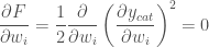
  to be the half squared error of
  .
.


 and
and  are learning rate hyperparameters.
 i.e. That it tends to 1 as x approaches positive infinity
 i.e. That it tends to 0 as x approaches negative infinity
 and
and 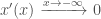
 .
.
 and
and 


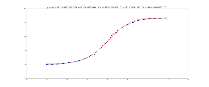
 then
then  . I was too lazy to update the graphs sorry)
 :
:
