Okay, so clickbait title, because I’m referring to the most common case of using a single Gaussian distribution to represent the current estimated position (for example) and for the measurement.

Here’s my problem with that:

They don’t take into account that sometimes things go wrong.

Now you may say ‘duh’, but it can cause some really serious problems if something does go wrong.

Say you have a self driving car.  And the following happens:

• Prior: You currently estimate the position of a person in front of you to be at position:  x = 2m ± 0.5m     aka   X ~ N(2,0.5)
• Data:  Your instruments return a new measure:  the person is now measured to be at position: x = 10m ± 0.5m   aka    X ~ N(10,0.5)
• Posterior: You apply your Kalman Filter and it concludes that the position of the person is now at:  x = 6m ± 0.25m  aka   X ~ N(6,0.25)

• You are now extremely confident that the person is at x=6m despite you previously thinking that they were at a x=2m and your measurement data says that they are at x=10m.  You, the self driving car, now happily drive at x=10m.

How confident would you, as a, human, really be that the person is at x=6m?  Barely at all, right?  So something has gone wrong here.

Here’s an example in a simulator.  A car is driving from right to left and we are trying to track its true position with a Extended Kalman Filter.  ◯ The red circles indicate data from the simulated LASER, ◔ blue circle circles are RADAR, and ▲ green triangles are the position estimated by a Kalman filter.  At the bottom of the arc, a single bad LASER data point is injected.

Credit to Udacity for the simulator.

The result is that the predicted position goes way off, and takes many times steps to recover.

The blame all lies on Sherlock Holmes:

The product of N(2,0.5) * N(10,0.5) results in a ridiculous improbable scenerio – we have to scale up the result by .  i.e. treating the highly improbable as truth.  Perhaps what Sherlock should have said is that it is far more likely that you were simply mistaken in elimination!  i.e. your prior or data was wrong!

Fixing the basic Kalman Filter

Here’s a small change we could make.  We can add a small probability of ‘wtf’ to our system.

• Prior: You currently estimate the position of a person in front of you to be at position:    plus a chance of ‘wtf’:   aka:
  
• Data:  Your instruments return a new measure:  the person is now measured to be at position:   plus a chance of ‘wtf’:   aka:
  
  
  
• Posterior: You apply your bayes rule.  What do we get now?  We need the product of these two random variables, and then normalize, by setting C such that the total integral is 1.(note that is proportionate to a new Gaussian scaled by a factor )
  We know that the area must equal 1 for a PDF, so we can determine the scale factor C.  See Appendix below for any technical details, including the formula for S and C.So we have a solution, but the solution is a gaussian mixture model – a sum of a gaussian for the combination, a gaussian for the prior, and a gaussian for the data.  So let’s simply pick the one with the highest probability, and roll the other two into the WTF weight.

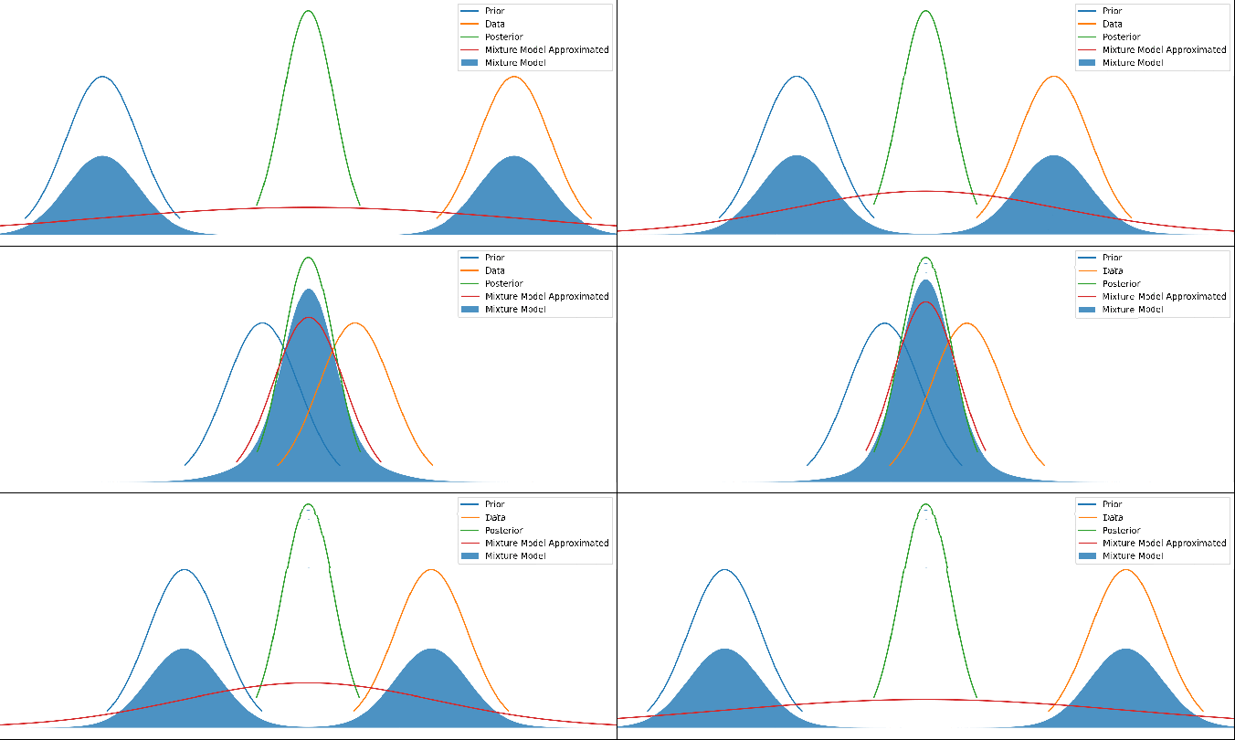
Here’s the result as an gif – the posterior is where the posterior would normally be, and the shaded blue area is our ‘wtf’ version of the posterior as a weighted mixture model:

Various different priors and data.  There’s no updating step here – just showing different mean values for the prior and data.  The posterior is kept centered to make it easier to see.

It looks pretty reasonable!  If the prior and data agree to within their uncertainties, then the mixture model just returns the posterior.  And when they disagree strongly, we return a mixture of them.

Let’s now make an approximation of that mixture model to a single gaussian, by choosing a gaussian that minimizes the KL divergence.

Which results in the red line ‘Mixture Model Approximated’:

Different priors and data, with the red line showing this new method’s output.  As above, there’s no update step here – it’s not a time series.

Now this red line looks very reasonable!  When the prior and data disagree with each other, we have a prediction that is wide and covers both of them.  But when they agree with each other to within their uncertainties, we get a result that properly combines both and gives us a posterior result that is more certain than either – i.e. we are adding information.

In total, the code to just take a prior and data and return a posterior is this:
(Note: I’ve assumed there are no covariances – i.e. no correlation in the error terms)

# prior input
mu1 = 5
variance1 = 0.5
# data input
mu2 = 6
variance2 = 0.5
# This is what you would normally do, in a standard Kalman Filter:
variance3 = 1/(1/variance1 + 1/variance2)
mu3 = (mu1/variance1 + mu2/variance2)*variance3

#But instead we will do:
S = 1/(np.sqrt(2*np.pi*variance1*variance2/variance3)) * np.exp(-0.5 * (mu1 - mu2)**2 * variance3/(variance1*variance2))
Wprior = 0.01 # 1% chance our prior is wrong
Wdata = 0.01 # 1% chance our data is wrong
C = (1-Wprior) * (1-Wdata) * S + (1-Wprior) * Wdata + Wprior * (1-Wdata)
weights = [
Wprior * (1-Wdata) /C, # weight of prior
(1-Wprior) * Wdata /C, # weight of data
(1-Wprior) * (1-Wdata) * S/C ] #weight of posterior
mu4 = weights[0]*mu1 + weights[1]*mu2 + weights[2] * mu3
variance4 = weights[0]*(variance1 + (mu1 - mu4)**2) + \
weights[1]*(variance2 + (mu2 - mu4)**2) + \
weights[2]*(variance3 + (mu3 - mu4)**2)

So at mu3 and variance3  is the green curve in our graphs and is the usual approach, while mu4 and variance4 is my new approach and is a better estimation of posterior.

The full ipython notebook code for everything produced here, is in git, here:

https://github.com/johnflux/Improved-Kalman-Filter/blob/master/kalman.ipynb

Results: Testing out in Simulator

Unfortunately, in my simulator my kalman filter has a velocity component, which I don’t actually take into in my analysis yet.  My math completely ignores any dependent variables.  The problem is that when we increase the uncertainty of the position then we also need to increase the uncertainty of the velocity.

To salvage this, I used just a small part of the code:

<div>
<div>double Scale = 1/(sqrt(2*M_PI*variance1*variance2/variance3)) * exp(-0.5 * (mu1 – mu2)*(mu1 – mu2) * variance3/(variance1*variance2));</div>
<div>
<div>
<div>if (Scale < 0.00000000001)
return; /* Just completely ignore this data point */</div>
</div>
</div>
</div>

The result is this:

Appendix:

Just some technical notes, for completeness.

• We can set where it can be anywhere between A and -A.  We can take A to be large or even take the limit to infinity.
• It is a Probability Density Function since the area is 1:  , and can set the Cauchy principal value of the integral to be 1 to keep it a PDF in the limit.
• since:    which tends to 0 as .
• The scale factor S is simple but tedious to calculate:
  
• The scale factor C can then be calculated by just setting the integral to equal 1 since it’s a PDF: 

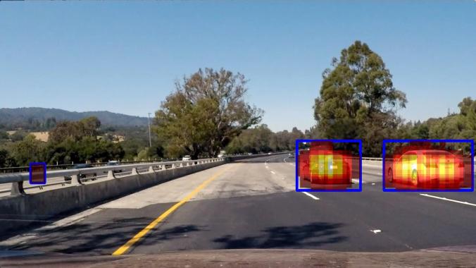
For my self-driving car, I detect cars in the image by scanning over the image in windows of varying sizes, and use the detection results to build up a ‘heat map’ of the most likely areas for where the cars are.

For visualization I came up with this idea:

In code:

heat_img = plt.cm.hot(heat/np.max(heat))
heat_img[heat<1,3] = 0 image2 = np.copy(image) image2[heat>1,:] = image2[heat>1,:]/3 + (heat_img[heat>1,0:3]*256*2/3).astype(np.uint8)
plt.imshow(image2)

Well, in a simulator 🙂

(Sorry about the bad filming – it was the easiest way to get even a semi-decent quality)

Code is here: https://github.com/johnflux/CarND-Behavioral-Cloning-P3

I basically follow the NVidia End to End Learning for Self-Driving Cars paper with a few tweaks to add in dropout, slightly larger Dense layers to compensate, and an additional convolution layer to handle the different input image resolution.  It runs in real time on a GTX 980 Ti.

I see people new to machine learning make the same sort of mistakes.  Mistakes that I’ve made myself and then painstakingly tried to fix.  So here’s some hints that I’ve had to work out the hard way, along with some code.

As an example, I’ve used my self driving car code, which I’ll put up on the web.

• Plot your input and expected output data!  For the training, validation and test data, individually.  It’s too easy to accidentally shuffle your data in the wrong place or to have unbalanced data etc.

  Example:

  def showDrivingAngles(samples, title="samples"):
      plt.hist([sample.driving_angle for sample in samples ], 16)
      plt.title("Driving angle distribution in " + title)
      plt.show()
  showDrivingAngles(samples)
  

• Make sure your data is balanced, by over-sampling, under-sampling or generating fake data.

  Example to over-sample:  (Suggestions on making this better are welcome!)

  def duplicateSamplesToRebalanceByDrivingAngle(samples):
      # Bin the data, returning an array of which bin each sample is in
      num_bins = 16
      indexes = np.digitize([sample.driving_angle for sample in samples], np.arange(-1, 1, 2/num_bins))
      # Find how many samples are in the largest bin
      largest_bin_count = np.max(np.bincount(indexes))
      print(largest_bin_count)
      rebalanced_samples = []
      for j in range(num_bins):
          bin_indexes = np.where(indexes==(j+1))[0]
              for i in range(largest_bin_count):
                  rebalanced_samples.append(samples[bin_indexes[i % len(bin_indexes)]])
      random.shuffle(rebalanced_samples)
      return rebalanced_samples
  

  (And of course, plot your data afterwards like above, to check that it worked correctly)

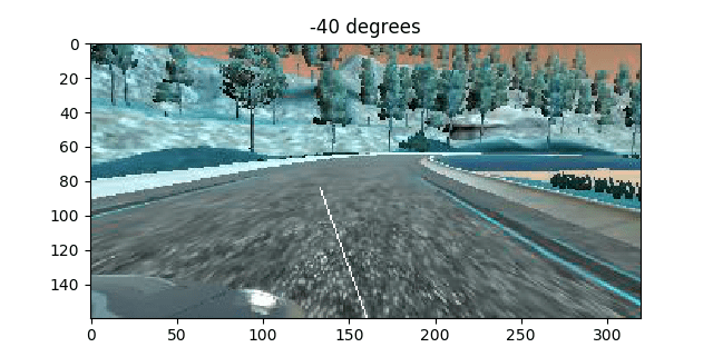
• View random samples of your data after preprocessing.  It’s worthwhile to get a bit fancy here.  Show the label for the data here.  For example, I draw an arrow directly on the image to indicate which direction the label says that it should go in:

  image = self.getImage()
   s = image.shape
   line_len = s[0]//2
   angle = self.driving_angle / 360 * np.pi * 100 # Times 100 just to make it more visible
   line_y, line_x = int(line_len * np.cos(angle)), int(line_len * np.sin(angle))
   rr,cc = draw.line(s[0]-1, s[1]//2, s[0]-1-line_y, s[1]//2 + line_x)
   image[rr,cc,:] = 255
   plt.imshow(image)
   plt.title("{} degrees".format(float(self.driving_angle)))
   plt.show()
  

  

• Check your colorspace! Notice that in the image above, the colors are all wrong. This was totally on purpose, to demonstrate another point – Make sure you understand what colorspace your data is in! cv2.imread() return BGR. While almost everything else is going to use RGB. I highly recommend converting to YUV immediately, and using that everywhere. Make sure you do this in both the code that trains the model, and code that uses the model.
• You can do preprocessing in the model itself.  This is extremely useful if you want to use your model in a program and don’t want to copy the preprocessing code.

  Example to crop and normalize image:

  inputs = keras.layers.Input(shape=(160,320,3))
  output = keras.layers.convolutional.Cropping2D(cropping=((55, 25), (0, 0)))(inputs)
  output = Lambda(lambda x: x/127.5 - 1., input_shape=imageshape, output_shape=imageshape)(output)
  

• If you do preprocess in the model, preview the output.  You can do this by creating a temporary model and using predict.
  Example:

  def showLayerOutput(sample):
      model = Model(inputs=inputs, outputs=output)
      sample.showImage()
      croppedimage = model.predict(np.array([sample.getImage()]))[0]
      print(croppedimage)
      plt.imshow(croppedimage)
      plt.show()
  showLayerOutput(train_samples[0])
  

• Use asserts on the shape of your model.  For example:

  assert output.shape[1:] == (1,31,64)
  

• Print out some outputs!  This is really important to keep an eye on what the predictions are.  Are they never negative when you want them to be?  Are they never larger than one when you want them to be?  (You’re using the wrong activation function on the last layer). Is it always outputting zero or similar (learning rate too high?)
  In keras you do this with a callback.

  Example:

  class DebugCallback(keras.callbacks.Callback):
      def on_epoch_end(self, batch, logs={}):
          samples = train_samples[:5]
          print()
          print(logs)
          print("Should be: ", [sample.driving_angle for sample in samples])
          print("Predicted: ", [x[0] for x in model.predict(np.array([sample.getImage() for sample in samples]))] ) #Print predicted driving angle for first example
  
  debugCallback = DebugCallback()
  model.fit_generator(train_generator, epochs=200, steps_per_epoch= len(train_samples)/batch_size, validation_data=validation_generator, validation_steps =len(validation_samples)/batch_size, callbacks=[tbCallBack, checkpointCallback, reduce_lr, debugCallback])
  

This is about a political post, but this post isn’t political but purely about the statistics.  A Lords Labour MP recently wrote:

We often read that there is a plus or minus 2 or 3% statistical margin of error in a poll. But what we are rarely reminded of is that this error applies to each party’s vote. So if a poll shows the Tories on 40% and Labour on 34%, this could mean that the real situation is Tory 43%, Labour 31% – a 12 point lead. Or it could mean both Tory and Labour are on 37%, neck and neck.

But is this true, mathematically?

When we say “Tories on 40% ± 3%”  we mean:

A Normal Distribution with mean 40, and standard deviation of 3/1.96

Let’s plot both on the same graph:

Which was achieved in Wolfram Alpha with:

Plot[{PDF[NormalDistribution[40, 3/1.96], x], 
      PDF[NormalDistribution[34, 3/1.96], x]},
      {x, 30, 44}]

Now, could Labour and Tory really be neck and neck, within our 95% confidence?

If they are not correlated at all, then no:

To subtract normal distributions you have to do:

so:

So, at 95% confidence, the difference in their lead is:  6 points ± 4.2.  As a plot:

The Neck-and-neck 0 point lead  and the 12 point lead are really unlikely outcomes! (0.3% in fact)

(Caveat:  Of course this all depends on the polls being accurate normal samples on the population).

But of course they are correlated… somewhat

If this was a two party system, with the total adding up to 100%, then the errors would be completely anti-correlated.  And if it was a many party system, with the total adding up to much less 100%, then we’d expect the errors to have a very weak correlation.  But with the errors adding up 70% we’re stuck in an awkward half-correlated stage.  Is there anything better that we can do?

Edit: Response from the Lords MP

I received a message from the MP:

I take your point but don’t entirely agree. The errors are associated ie high Tory is likely to mean low Labour and vice versa so these are linked contingencies.
But thanks for writing. And at least even if your point was accepted entirely it wouldn’t make any material difference to the conclusions of my article.
D

(This post is a work in progress, sorry. I’ll write it up better a bit later, honest!)

After a weekend of hacking around, I got a 95% accuracy rate on the validation and testing sets for recognizing road signs.  Here’s 5 random google images for ‘road sign photos’, and including one that fails:

My neural network got 4 out of 5 of the signs correct, incorrectly thinking the first image was 120 km/h instead of 20 km/h.  But it gets it correct on its second guess.

This was done by just adapting the LeNet neural network for recognizing digits.  I did add two dropout layers with a 50% probability, and increased the number of classes to 30 and input size to 32x32x3, and that was about it.

I had 35,000 training images, but increased this to 60,000 images by rotating and zooming the images.  My network does overfit badly though (reaching 99% accuracy on the training set, after 10 epochs).

This is using the very latest TensorFlow tf.contrib.learn API.  The documentation is extremely thin, and as of writing there are no tutorials out there similar to this.  The API may change, and I don’t actually know if I’m doing things correctly.  This is just trial and error 🙂

So let’s say you want to:

1. Train a Deep Neural Network by using some existing data, and training it against known labels.  e.g. labeled images.
2. Use that trained network in your app to predict y given x.  E.g. guess the best label for a given image

   And as a bonus:

3. Have some nice graphs of how well the training is doing

I assume that the data you have in a plain array-of-arrays or numpy 2D array.  It should be easy to change this to use csv or panda etc data. A row is a single example, and a column is a particular feature (e.g. house price, or pixel intensity at a specific location)

So, without further ado, here’s the function that will be shared between your training and your app

def get_tf_model():
    """ Setup our Deep Neural Network and LOAD any existing model
       
        Returns:
          ( Our (maybe trained) model, a helper input function)
    """
    # FEATURES is a short description for each column
    # of your data.  Change this to match your data
    FEATURES = ["x1", "x2"]
    # Set this to describe your columns.  If they are all real values,
    # you don't need to change it.
    feature_columns = [tf.contrib.layers.real_valued_column(k) for k in FEATURES]

    # Build 3 layer DNN.  You can change this however you want, or use a
    # linear regressor, or use a classifier etc.
    # NOTE:
    #   This will LOAD any existing model in the "model_dir" directory!
    # The documentation fails to mention this point as of writing
    regressor = tf.contrib.learn.DNNRegressor(feature_columns=feature_columns,
                                              hidden_units=[128, 128, 128],
                                              model_dir="tf_model")

    def input_fn(x_data, y_data = None):
        # Note the 'shape' parameter is to suppress a very noisy warning.
        # You can probably remove this parameter in a month or two.
        feature_cols = {k: tf.constant(x_data[:,i], shape=[len(x_data[:,i]), 1])
                        for i, k in enumerate(FEATURES)}
        if y_data is None:
            return feature_cols
        labels = tf.constant(y_data)
        return feature_cols, labels

    return regressor, input_fn

x_test = None
y_test = None
regressor, input_fn = get_tf_model()

def train(training_data_y, training_data_x):
    global x_test, y_test, regressor, input_fn

    if x_test is None:
        x_train = np.array(training_data_x[:-20], dtype=np.float32)
        x_test = np.array(training_data_x[-20:], dtype=np.float32)
        y_train = np.array(training_data_y[:-20], dtype=np.float32)
        y_test = np.array(training_data_y[-20:], dtype=np.float32)
    else:
        x_train = np.array(training_data_x, dtype=np.float32)
        y_train = np.array(training_data_y, dtype=np.float32)

    print("Training model ...")
    # Fit model.
    regressor.fit(input_fn=lambda: input_fn(x_train, y_train), steps=2000)

    ev = regressor.evaluate(input_fn=lambda: input_fn(x_test, y_test), steps=1)
    print('  -  Trained Loss: {0:f}'.format(ev["loss"]))

regressor, input_fn = get_tf_model()
def predict(x_data):
    return regressor.predict(input_fn=lambda:input_fn(x_data))

tensorboard tf_model  # or whatever you set model_dir to