Unity vs Unreal Engine 4

May 29, 2016December 19, 2016 / John Tapsell / 1 Comment

I implemented two medium-sized projects, one in Unreal Engine 4 and one in Unity 5.

Unfortunately these were both for clients, so I can’t talk about any specifics. I do, however, want to give some general thoughts on the comparison between them.

Pros and Cons:

Unreal Engine 4 seems to have a lot more advanced features. But I didn’t personally use any of these advanced features. They didn’t seem easy to use.
Unity 5 was much more intuitive for me to use.
The Unity 5 asset store was so much nicer to use. I could buy an asset and import it into my game with a couple of clicks. With UE4 it seemed so much more difficult.
UE4’s VR support simply didn’t work on a Mac. This sucked because my artists all use Macs. More annoyingly, it didn’t say why it didn’t work, it just simply disabled the Preview In VR button, giving no reason. And the reasons were written up in an Internal bug report (UE-11247 apparently) that the UE4 developers constantly refer to, but users aren’t actually allowed to view or see the status of!
I much preferred having a managed language (C# or javascript) in Unity than the C++ support in UE4. Mistakes in C++ code meant crashing the whole app. It also led to long compile times. But a mistake in C# meant just having an exception and the app being able to easily recover from it.
I tried really hard to get on with UE4’s Blueprint, which is basically a visual “programming” language. But implementing in a fairly simply mathematical formula would result in 20+ nodes. Implementing a simple polynomial like $latex y = 3x^2 + 2x + 5 $ was incredibly painful in dragging out nodes for each operation.

Blueprint quickly becomes a mess. This is a random example from the web.

UE4’s blueprints become particularly annoying when users are asking questions about them. They’ll paste a screenshot of their blueprint saying that they have a problem. Someone else then has to try to decipher what is going on from a screenshot, with really no easy way to reproduce. Users who want to copy a blueprint have to do so manually, node by node..
I would really love for UE4 to mix in a scripting language, like Javascript.
UE4 has lots of cool features, but they are really difficult to just use. For example, it has a lot of support for adding grass. You can just paint grass onto your terrain.. except that you can’t because you don’t have any actual grass assets by default.
The official UE4 tutorials say that to add grass, you should import the whole 6.4 GB Open World Demo Collection to your project!
But then, even that isn’t enough because it doesn’t have any actual grass materials! You have to then create your own grass material which is quite a long process. This was really typical of my experience with UE4. Why not just have a single ‘grass’ asset that could be instantly used, and then let the user tweak it in more complicated ways if they want to later on?
Compare this to Unity. You go to: Assets > Import Package > Terrain Assets click on the tree or grass that you want, and that’s it. You can then start painting with that tree or grass immediately. If you later want to make your own trees, it comes with a tree editor, built in!
Unity’s support for Android was much better than UE4’s.
UE4 taxed my system a lot more than Unity. For my beefy desktop, that was no problem. But the artists had Mac laptops that really struggled.
I really like Unity’s GameObject plus Component approach. Basically, you make a fairly generic GameObject that is in your scene, and then you attach multiple components to it. For example, if you want a button, your button GameObject would have a mesh, a material, a renderer (to draw the material on the mesh), a hit box (to know when the user presses it) and presumably some custom script component that runs when you hit it.
And because your custom scripts are written in C# or javascript, you get lovely automatically introspection on the class variables, and any variables are automatically added to the GUI!

Overall, I guess I’ve become a unity fanboy. Which is a shame, because I started with UE4 and I really wanted to like it. I have been with UE4 for 2 years, and was a paying sponsor for a year.

I feel that the trouble is their different audiences. UE4 is obviously targeted towards much larger studios, who want advanced features and don’t care about built in assets etc. Unity on the other hand is targeted towards Indie developers who want to make quick prototypes and cheap products easily.

This has resulted into a sort of stigma against Unity projects, because there is a glut of rubbish games produced by novices in Unity. Unity charges about $1,500 per developer to remove the start-up Unity splashscreen, resulting in most indie developers not paying that fee. Only the good games which sell well can afford to remove that splashscreen.

The result being that if you start up a random indie game on steam greenlight, for example, and see the Unity splashscreen, you know that the game is unlikely to be that good. Hence a stigma.

Logistic Regression and Regularization

May 20, 2016December 19, 2016 / John Tapsell / Leave a comment

Tons has been written about regularization, but I wanted to see it for myself to try to get an intuitive feel for it.

I loaded a dataset from google into python (a set of images of letters) and implemented a double for-loop to run a logistic regression with different test data sizes, and different regularization parameters. (The value shown in the graph is actually $1/regularization$ ).

def doLogisticRegression(trainsize, regularizer):
    fitmodel = linear_model.LogisticRegression(C=regularizer)
    train_datasubset = train_dataset[0:trainsize,:,:].reshape(trainsize, -1)
    x = fitmodel.fit(train_dataset[0:trainsize,:,:].reshape(trainsize, -1),
                 train_labels[0:trainsize])
    return [fitmodel.score(train_datasubset, train_labels[0:trainsize]),
            fitmodel.score(valid_dataset.reshape(valid_dataset.shape[0], -1), valid_labels)
            ]
print(train_dataset.shape[0])
trainsizes = [50,200,300,400,500,600,700,800,900,1000,2000,3000,4000,5000, 10000, 50000, 100000, 200000];
plt.xscale('log')
color = 0
plots = []
for regularizer in [1, 0.1, 0.01, 0.001]:
    results = np.array([doLogisticRegression(x, regularizer) for x in trainsizes])
    dashedplot = plt.plot(trainsizes, results[:,1], '--', label=(&amp;quot;r:&amp;quot; + str(regularizer)))
    plt.plot(trainsizes, results[:,0], c=dashedplot[0].get_color(), label=(&amp;quot;r:&amp;quot; + str(regularizer)))
    plots.append(dashedplot[0])
plt.legend(loc='best', handles=plots)

The result is very interesting. The solid line is the training set accuracy, and the dashed line is the validation set accuracy. The vertical axis is the accuracy rate (percentage of images recognized as the correct letter) and the horizontal axis is the number of training examples.

graph of accuracy against training set for logistic regression

Image to letter recognition accuracy against training size, for various values of r = 1/regularization_factor. Solid line is training set accuracy, dotted line is validation set accuracy.

First, I find it fascinating that purely a logistic regression can produce an accuracy of recognizing letters at 82%. If you added in spell checking, and ran this over an image, you could probably get a pretty decent OCR system, from purely an logistical regression.

Second, it’s interesting to see the effect of the regularization term. At less than about 500 training examples, the regularization term only hurts the algorithm. (A value of 1 means no regularization). At about 500 training examples though, the strong regularization (really helps). As the number of training examples increases, regularization makes less and less of an impact, and everything converges at around 200,000 training samples.

It’s quite clear at this point, at 200,000 training samples, that we are unlikely to get more improvements with more training samples.

A good rule of thumb that I’ve read is that you need approximately 50 training samples per feature. Since we have 28×28 = 784 features, this would be at 40,000 training samples which is actually only a couple of percent from our peak performance at 200,000 training samples (which is 2000000/784=2551 training samples per feature).

At this point, we could state fairly confidently that we need to improve the model if we want to improve performance.

Stochastic Gradient Descent

I reran with the same data but with stochastic gradient descent (batch size 128) and no regularization. The accuracy (after 9000 runs) on the validation set was about the same as the best case with the logistic regression (81%), but took only a fraction of the time to run. It took just a few minutes to run, verses a few hours for the logistic regression.

Stochastic Gradient Descent with 1 hidden layer

I added a hidden layer (of size 1024) and reran. The accuracy was only marginally better (84%). Doubling the number of runs increased this accuracy to 86%.

Exploiting internal neural network symmetries

May 19, 2016December 19, 2016 / John Tapsell / Leave a comment

Neural networks have many internal symmetries. A symmetry is an operation that you can apply to the weights such that for all inputs the outputs are the same.

The trivial symmetry is the identity. If you multiply all the weights in a neural network by 1, then the output remains unchanged.

We can also move nodes around by swapping the weight in any hidden layer. For example:

Diagram1

But what other symmetries are there? How is this useful?

Well, by itself, it’s not. But let’s get hand-wavy. Let’s say that we are using a ReLU activation function. What this means is that at our hidden node, if the final value is greater than 0, then the output at that node is the same value. if it’s negative, then the output is 0.

Let’s hand wave like crazy, and consider only the case where the node is activated (i.e the total value going into node is >=0). The output is equal to the input, and in this region it is linear.

So, ignoring the non-linear case, we can find an interesting symmetry. We can project to the basis $[1,1]/\sqrt{2}$ and $[1,-1]/\sqrt{2}$ . Or in pictures:

Diagram2

So, ignoring the non-linearity at the hidden layer, we find that we can actually weights in a more interesting fashion.

Now, what can we do with this?

Honestly, I’m not sure. One idea I had is if you’ve optimized a neural net and reached the peak that your training set can give you, you could apply this swap operation to random nodes and retrain and see if it helps. The effect is that you’re leaving the weights the same, but changing when the node activates. Hopefully I’ll have a better idea later.

Meta Neural Network

April 4, 2016December 19, 2016 / John Tapsell / Leave a comment

The idea is to create a large neural network which itself generates other neural networks. The goal is to let the neural network find a way to just create new networks without any training needed.

I have two very different ideas on how to do this.

The first is not so practical to implement for any real world problems, but would be interesting to test on toy problems:

meta neural net idea

Now, this idea has many drawbacks. One problem is that when training the “Author” network in the first place, you typically have a fixed size input and so the training input will need to have a fixed size.

Since the input needs to be a fixed size, this means that you are limited to fixed size input and output for all the “Baby” Neural Networks that are generated, and that you must always have the same number of training samples.

Likewise, since the output is a fixed size, the weights has to be a fixed size, and so the number of layers, size of the layers, architecture, and so on has to be fixed for all possible Baby networks generated for a given Author.

Four point gradient as a GLSL shader

March 16, 2016March 24, 2016 / John Tapsell / Leave a comment

For a client I needed a way to draw a gradient in realtime generated from four points, on a mobile phone. To produce an image like this, where the four gradient points can be moved in realtime:

I wanted to implement this using a shader, but after googling for a while I couldn’t find an existing implementation.

The problem is that I have the desired colours at four points, and need to calculate the colour at any other arbitrary point.

So we have three simultaneous equations (vectors in bold):

$\begin{array} {ccccc} \boldsymbol{A} &=& \boldsymbol{P_0} (1-u) &+& \boldsymbol{P_1} u \\ \boldsymbol{B} &=& \boldsymbol{P_2} (1-v) &+& \boldsymbol{P_3} v \\ \boldsymbol{C} &=& \boldsymbol{A} (1-t) &+& \boldsymbol{B} t \end{array}$

The key to solving this is to reduce the number of freedoms by setting $u = v$ .

$\begin{array} {ccccc} \boldsymbol{A} &=& \boldsymbol{P_0} (1-u) &+& \boldsymbol{P_1} u \\ \boldsymbol{B} &=& \boldsymbol{P_2} (1-u) &+& \boldsymbol{P_3} u \\ \boldsymbol{C} &=& \boldsymbol{A} (1-t) &+& \boldsymbol{B} t \end{array}$

Solving for $t$ gives us:

$(\boldsymbol{A-B})t = (\boldsymbol{A-C})$

And solving for $\boldsymbol{A}$ and $\boldsymbol{B}$ :

$\begin{array} {ccl} \boldsymbol{A} &=& \boldsymbol{P_0} (1-u) + \boldsymbol{P_1}(u)\\ &=& \boldsymbol{P_0} + u(\boldsymbol{P_1} - \boldsymbol{P_0})\\ \boldsymbol{B} &=& \boldsymbol{P_2} (1-u) + \boldsymbol{P_3}(u)\\ &=& \boldsymbol{P_2} + u(\boldsymbol{P_3} - \boldsymbol{P_2}) \end{array}$

so:

$\boldsymbol{A}-\boldsymbol{B} = \boldsymbol{P_0} - \boldsymbol{P_2} + u(\boldsymbol{P_1} - \boldsymbol{P_0} + \boldsymbol{P_2} - \boldsymbol{P_3}) \Rightarrow \\\\ (\boldsymbol{P_0} - \boldsymbol{P_2} + u(\boldsymbol{P_1} - \boldsymbol{P_0} + \boldsymbol{P_2} - \boldsymbol{P_3}))t = \boldsymbol{P_0} + u(\boldsymbol{P_1} - \boldsymbol{P_0}) - \boldsymbol{C}\\$

Defining:

Lets us now rewrite $(\boldsymbol{A-B})t = (\boldsymbol{A-C})$ as:

$(\boldsymbol{Q} + u\boldsymbol{S})t = \boldsymbol{T} + u\boldsymbol{R}$

Which written out for x and y is:

$(Q.x + u S.x)t = T.x + uR.x\\ (Q.y + u S.y)t = T.y + uR.y$

Now we have to consider the various different cases. If $Q.x == 0\ \&\&\ S.x == 0$ then we have:

$u = -T.x/R.x\\ t = (T.y + uR.y) / (Q.y + u S.y)$

Likewise if $Q.y == 0\ \&\&\ S.y == 0$ then we have:

$u = -T.y/R.y\\ t = (T.x + uR.x) / (Q.x + u S.x)$

Otherwise we are safe to divide by $(Q.y + u S.y)$ and so:

$\\ (Q.x + u S.x)/(Q.y + u S.y) = (T.x + uR.x)/(T.y + uR.y)\\ \\ (Q.x + u S.x)(T.y + uR.y) = (T.x + uR.x)(Q.y + u S.y)\\ \\ (Q.x + u S.x)T.y +(Q.x + u S.x) uR.y = (T.x + uR.x)Q.y + (T.x + uR.x)u S.y\\ \\ Q.x T.y + u S.x T.y +Q.x uR.y + u S.x uR.y = T.x Q.y + uR.x Q.y + T.x u S.y + uR.x u S.y\\ \\ Q.x T.y - T.x Q.y + u (S.x T.y - T.x S.y + Q.x R.y - R.x Q.y) + u^2 (S.x R.y - R.x S.y) = 0\\ \\ A := S.x R.y - R.x S.y\\ B := S.x T.y - T.x S.y + Q.x R.y - R.x Q.y\\ C := Q.x T.y - T.x Q.y\\ \\ A u^2 + B u + C = 0\\$

Which can be solved with the quadratic formula when A is not zero: (Note that only the positive solution makes physical sense for us, and we can assume $A \neq 0$ )
$u = \dfrac{-B+\sqrt{B^2 - 4AC}}{2A}$

and when A is zero (or, for computational rounding purposes, close to zero):

$u = \dfrac{-B}{C}$

Math Summary

We can determine $u$ and $t$ with:

$\begin{array} {ccl} \boldsymbol{Q} &=& \boldsymbol{P_0} - \boldsymbol{P_2}\\ \boldsymbol{R} &=& \boldsymbol{P_1} - \boldsymbol{P_0}\\ \boldsymbol{S} &=& \boldsymbol{R} + \boldsymbol{P_2} - \boldsymbol{P_3}\\ \boldsymbol{T} &=& \boldsymbol{P_0} - \boldsymbol{C}\\ A &:=& S.x R.y - R.x S.y\\ B &:=& S.x T.y - T.x S.y + Q.x R.y - R.x Q.y\\ C &:=& Q.x T.y - T.x Q.y\\ u &=& \begin{cases} -T.x/R.x, & \mbox{if } \mbox{ Q.x == 0.0\ \&\&\ S.x == 0.0} \\ -T.y/R.y, & \mbox{if } \mbox{ Q.y == 0.0\ \&\&\ S.y == 0.0} \\ \dfrac{-B}{C}, & \mbox{if A == 0} \\ \dfrac{-B+\sqrt{B^2 - 4AC}}{2A}, & \mbox{otherwise} \\ \end{cases} \\\\ t &=& \begin{cases} \dfrac{T.y + u R.y}{Q.y + u S.y}, & \mbox{if } \mbox{ Q.x == 0.0\ \&\&\ S.x == 0.0} \\ \dfrac{T.y + u R.y}{Q.y + u S.y}, & \mbox{otherwise} \\ \end{cases} \end{array}$

Implementation as a shader:

This can be implemented as a shader as following: (The following can be run directly on https://www.shadertoy.com for example)

void mainImage( out vec4 fragColor, in vec2 fragCoord )
{

    //Example colors.  In practise these would be passed in
    // as parameters
    vec4 color0 = vec4(0.918, 0.824, 0.573, 1.0); // EAD292
    vec4 color1 = vec4(0.494, 0.694, 0.659, 1.0); // 7EB1A8
    vec4 color2 = vec4(0.992, 0.671, 0.537, 1.0); // FDAB89
    vec4 color3 = vec4(0.859, 0.047, 0.212, 1.0); // DB0C36

    vec2 uv = fragCoord.xy / iResolution.xy;

    //Example coordinates.  In practise these would be passed in
    // as parameters
    vec2 P0 = vec2(0.31,0.3);
    vec2 P1 = vec2(0.7,0.32);
    vec2 P2 = vec2(0.28,0.71);
    vec2 P3 = vec2(0.72,0.75);

    vec2 Q = P0 - P2;
    vec2 R = P1 - P0;
    vec2 S = R + P2 - P3;
    vec2 T = P0 - uv;

    float u;
    float t;

    if(Q.x == 0.0 &amp;amp;&amp;amp; S.x == 0.0) {
        u = -T.x/R.x;
        t = (T.y + u*R.y) / (Q.y + u*S.y);
    } else if(Q.y == 0.0 &amp;amp;&amp;amp; S.y == 0.0) {
        u = -T.y/R.y;
        t = (T.x + u*R.x) / (Q.x + u*S.x);
    } else {
        float A = S.x * R.y - R.x * S.y;
        float B = S.x * T.y - T.x * S.y + Q.x*R.y - R.x*Q.y;
        float C = Q.x * T.y - T.x * Q.y;
        // Solve Au^2 + Bu + C = 0
        if(abs(A) < 0.0001)
            u = -C/B;
        else
	    u = (-B+sqrt(B*B-4.0*A*C))/(2.0*A);
        t = (T.y + u*R.y) / (Q.y + u*S.y);
    }
    u = clamp(u,0.0,1.0);
    t = clamp(t,0.0,1.0);

    // These two lines smooth out t and u to avoid visual 'lines' at the boundaries.  They can be removed to improve performance at the cost of graphics quality.
    t = smoothstep(0.0, 1.0, t);
    u = smoothstep(0.0, 1.0, u);

    vec4 colorA = mix(color0,color1,u);
    vec4 colorB = mix(color2,color3,u);
    fragColor = mix(colorA, colorB, t);
}

And the same code again, but formatted as a more typical shader and with parameters:

          uniform lowp vec4 color0;
          uniform lowp vec4 color1;
          uniform lowp vec4 color2;
          uniform lowp vec4 color3;
          uniform lowp vec2 p0;
          uniform lowp vec2 p1;
          uniform lowp vec2 p2;
          uniform lowp vec2 p3;
          varying lowp vec2 coord;

          void main() {
            lowp vec2 Q = p0 - p2;
            lowp vec2 R = p1 - p0;
            lowp vec2 S = R + p2 - p3;
            lowp vec2 T = p0 - coord;

            lowp float u;
            lowp float t;

            if(Q.x == 0.0 &amp;amp;&amp;amp; S.x == 0.0) {
                u = -T.x/R.x;
                t = (T.y + u*R.y) / (Q.y + u*S.y);
            } else if(Q.y == 0.0 &amp;amp;&amp;amp; S.y == 0.0) {
                u = -T.y/R.y;
                t = (T.x + u*R.x) / (Q.x + u*S.x);
            } else {
                float A = S.x * R.y - R.x * S.y;
                float B = S.x * T.y - T.x * S.y + Q.x*R.y - R.x*Q.y;
                float C = Q.x * T.y - T.x * Q.y;
                // Solve Au^2 + Bu + C = 0
                if(abs(A) < 0.0001)
                    u = -C/B;
                else
                    u = (-B+sqrt(B*B-4.0*A*C))/(2.0*A);
                t = (T.y + u*R.y) / (Q.y + u*S.y);

            }
            u = clamp(u,0.0,1.0);
            t = clamp(t,0.0,1.0);

            // These two lines smooth out t and u to avoid visual 'lines' at the boundaries.  They can be removed to improve performance at the cost of graphics quality.
            t = smoothstep(0.0, 1.0, t);
            u = smoothstep(0.0, 1.0, u);

            lowp vec4 colorA = mix(color0,color1,u);
            lowp vec4 colorB = mix(color2,color3,u);
            gl_FragColor = mix(colorA, colorB, t);
          }

Result

On the left is the result using smoothstep to smooth t and u, and on the right is the result without it. Although the non-linear smoothstep is computationally-expensive and a hack, I wasn’t happy with the visual lines that resulted in not using it.

Lego

February 4, 2016December 19, 2016 / John Tapsell / Leave a comment

A quick break from any serious posts 🙂

First a LEGO bridge that I put together, held up by the tension in the inverted catenary suspension ‘rope’. It’s surprisingly sturdy – it can be picked up and moved without danger of breaking – the tension gives it quite a bit of strength.

Lego suspension bridge

And next a tower.

I starting running out of LEGO and so had to resort to balancing it on LEGO trees.

Isosceles Trapezoid

I made this after fiddling with the blocks and realising that I can quite significantly increase the sturdiness of a tower by forcing the LEGO blocks to connect an angle to make a trapezoid shape. I played about with different shapes and angles to maximize strength. The result looks very slapdash, but it’s surprisingly strong.

Tower

Long Short Term Memory

January 31, 2016December 19, 2016 / John Tapsell / 1 Comment

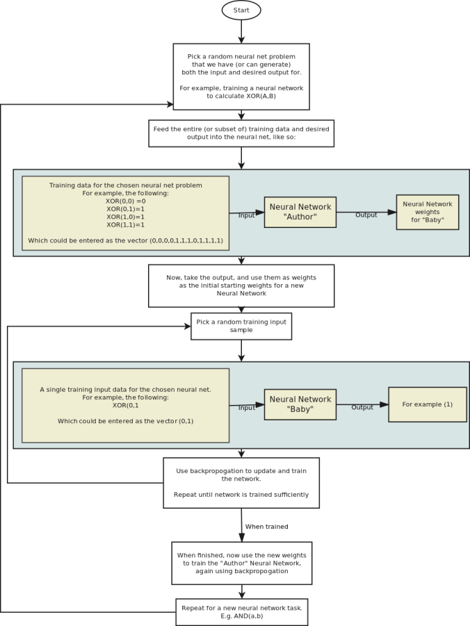
LSTM Neural Networks are interesting. There’s plenty of literature on the web about them, so I thought I’d cut to the chase and show how to implement a toy game.

In this game, we want to have a mouse and a cat in a room. The cat tries to eat the mouse, and the mouse tries to avoid being eaten.

Cat & Mouse start randomly. Mouse is taught to run away from the stationary cat.

We will give the mouse and cat both an LSTM Neural Network brain, and let them fight it out.

This game will be implemented with a straight forward LSTM neural network. This means that it is supervised which means that our mouse and cat brains can only learn by example.

This is really important – it means that we can’t just have our mouse and cat learn for themselves. We could do that if we used genetic algorithms to develop the neural networks, but that’s not how we’re doing it here.

With all that said, let’s just dive straight in!

First, lets set up a sigmoid function and its derivative:

#!/usr/bin/python
import copy, numpy as np
import math
np.random.seed(0)

# compute sigmoid nonlinearity
def sigmoid(x):
    output = 1/(1+np.exp(-x))
    return output

# convert output of sigmoid function to its derivative
def sigmoid_output_to_derivative(output):
    return output*(1-output)
class LSTM_Brain:
    def __init__(self):
        self.alpha = 0.1         # Training rate
        self.input_dim = 4       # Number of parameters for the input.  We input the position of the cat and the mouse.
        self.hidden_dim = 16     # Size of a brain, so to speak.  Feel free to vary
        self.output_dim = 1      # Number of outputs.  We output just the preferred direction, so just one.
        self.brain_wipe()

    def setupTraining(self):
        self.input_values = list()
        self.layer_2_deltas = list()
        self.layer_1_values = list()
        self.layer_1_values.append(np.zeros(self.hidden_dim))
        self.total_abs_error = 0  # Store the error and smoothed error just for debugging information

    def feedInputForGetOutput(self, inputData):
        # inputData has only been tested for values between 0 and 1.  Not sure how it works otherwise
        assert len(inputData) == self.input_dim
        X = np.array([inputData])
        self.input_values.append(X)
        # Feed the input to our 'brain', and return the output (e.g. which direction it thinks we should move in)
        # hidden layer (input ~+ prev_hidden)
        layer_1 = sigmoid(np.dot(X,self.synapse_0) + np.dot(self.layer_1_values[-1],self.synapse_h))
        # output layer (new action)
        self.layer_2 = sigmoid(np.dot(layer_1,self.synapse_1))
        # store hidden layer so we can use it in the next timestep
        self.layer_1_values.append(copy.deepcopy(layer_1))
        return self.layer_2[0]

    def teachError(self, error):
        self.total_abs_error += sum(np.abs(error))  # We store this just for debugging
        self.layer_2_error = np.array([error]).T
        self.layer_2_deltas.append((self.layer_2_error)*sigmoid_output_to_derivative(self.layer_2))

    def brain_wipe(self):
        # initialize neural network weights.  Forget everything we've learned
        self.synapse_0 = 2*np.random.random((self.input_dim,self.hidden_dim)) - 1
        self.synapse_1 = 2*np.random.random((self.hidden_dim,self.output_dim)) - 1
        self.synapse_h = 2*np.random.random((self.hidden_dim,self.hidden_dim)) - 1
        self.total_smoothed_abs_error = None

    def learnFromGame(self):
        future_layer_1_delta = np.zeros(self.hidden_dim)
        synapse_0_update = np.zeros_like(self.synapse_0)
        synapse_1_update = np.zeros_like(self.synapse_1)
        synapse_h_update = np.zeros_like(self.synapse_h)

        # Now, learn from the game
        for time_tick in range(len(self.input_values)):
            X = self.input_values[-time_tick-1]

            layer_1 = self.layer_1_values[-time_tick-1]
            prev_layer_1 = self.layer_1_values[-time_tick-2]

            # error at output layer
            layer_2_delta = self.layer_2_deltas[-time_tick-1]
            # error at hidden layer
            layer_1_delta = (future_layer_1_delta.dot(self.synapse_h.T) + layer_2_delta.dot(self.synapse_1.T)) * sigmoid_output_to_derivative(layer_1)

            # let's update all our weights so we can try again
            synapse_1_update += np.atleast_2d(layer_1).T.dot(layer_2_delta)
            synapse_h_update += np.atleast_2d(prev_layer_1).T.dot(layer_1_delta)
            synapse_0_update += X.T.dot(layer_1_delta)

            future_layer_1_delta = layer_1_delta

        self.synapse_0 += synapse_0_update * self.alpha
        self.synapse_1 += synapse_1_update * self.alpha
        self.synapse_h += synapse_h_update * self.alpha

        if self.total_smoothed_abs_error is None:
            self.total_smoothed_abs_error = self.total_abs_error
        else:
            self.total_smoothed_abs_error = self.total_smoothed_abs_error * 0.999 + 0.001* self.total_abs_error  # Smooth it - for debugging only

At this point, we’ve got a basic LSTM.

Let’s now give it a world and put this brain in a mouse, and the mouse in a world.

class World:
    # For directions, 0,0 is in the bottom left.  Up is positive y.  Direction is between 0 and 1
    Up = 0.125
    Right = 0.375
    Down = 0.625
    Left = 0.875

    def __init__(self):
        self.map_width = 6
        self.map_height = 6

    def resetWorld(self, cat_x, cat_y, mouse_x, mouse_y):
        self.cat_x = cat_x
        self.cat_y = cat_y
        self.mouse_x = mouse_x
        self.mouse_y = mouse_y

    def distance_from_cat_x(self):
        return self.mouse_x - self.cat_x
    def distance_from_cat_y(self):
        return self.mouse_y - self.cat_y

    def moveMouse(self, time_tick, mouse_movement):
        if mouse_movement &lt; (self.Up + 0.125):   # 0 to 0.25 is up.  midpoint is 0.125
            self.mouse_y += 1
        elif mouse_movement &lt; (self.Right + 0.125):  # 0.25 to 0.5 is right.  midpoint is 0.375
            self.mouse_x += 1
        elif mouse_movement &lt; (self.Down + 0.125): # 0.5 to 0.75 is down.  midpoint is 0.625
            self.mouse_y -= 1
        else:
            self.mouse_x -= 1   # 0.75 to 1 is left.  midpoint is 0.875
        self.mouse_x = np.clip(self.mouse_x, 0, self.map_width-1)
        self.mouse_y = np.clip(self.mouse_y, 0, self.map_height-1)

class GameWithStupidComputerTeacher:
    def __init__(self):
        self.debug = False     # Whether to print out debug information
        self.game_length = 10  # Number of moves a game should last for.  We make this fixed, but we could make it variable
        self.world = World()   # The world to run in

    def runGame(self, mouse_brain):
        # Start a new game.  We have a cat and a mouse
        # at their starting position
        self.world.resetWorld(np.random.randint(0,self.world.map_width),np.random.randint(0,self.world.map_height),
                              np.random.randint(0,self.world.map_width),np.random.randint(0,self.world.map_height))

        mouse_brain.setupTraining()

        for time_tick in range(self.game_length):
            mouse_movement = mouse_brain.feedInputForGetOutput([(self.world.cat_x)/float(self.world.map_width-1),
                                                                (self.world.cat_y)/float(self.world.map_width-1),
                                                                (self.world.mouse_x)/float(self.world.map_height-1),
                                                                (self.world.mouse_y)/float(self.world.map_height-1)])[0]

            ideal_direction = self.stupidTeacherForMouseGetIdealDirection()
            mouse_brain.teachError([ideal_direction - mouse_movement])

            # This is the direction the mouse brain says it wants to move in.  We treat it as a clockwise compass reading
            # Move the mouse accordingly
            #self.world.moveMouse(time_tick, ideal_direction)
            self.world.moveMouse(time_tick, mouse_movement)

        # Game is completed.  Learn from what we've been taught.
        mouse_brain.learnFromGame()

    def stupidTeacherForMouseGetIdealDirection(self):
        # Play the role of a stupid teacher for the mouse, and direct the mouse to just run in the opposite direction from the cat
        ideal_direction = 0
        if self.world.distance_from_cat_x() &gt;= 0:
            # We could move right.  But check if moving up or down makes more sense
            if self.world.distance_from_cat_y() &gt; self.world.distance_from_cat_x() and self.world.mouse_y != self.world.map_height - 1:
                ideal_direction = self.world.Up
            elif -self.world.distance_from_cat_y() &gt; self.world.distance_from_cat_x() and self.world.mouse_y != 0:
                ideal_direction = self.world.Down
            elif self.world.distance_from_cat_y() &gt; 0 and self.world.mouse_x == self.world.map_width - 1:
                ideal_direction = self.world.Up
            elif self.world.distance_from_cat_y() &lt; 0 and self.world.mouse_x == self.world.map_width - 1:
                ideal_direction = self.world.Down
            else:
                ideal_direction = self.world.Right
        else:
            if self.world.distance_from_cat_y() &gt; -self.world.distance_from_cat_x() and self.world.mouse_y != self.world.map_height - 1:
                ideal_direction = self.world.Up # up is the best way!
            elif -self.world.distance_from_cat_y() &gt; -self.world.distance_from_cat_x() and self.world.mouse_y != 0:
                ideal_direction = self.world.Down # down is the best way!
            elif self.world.distance_from_cat_y() &gt;= 0 and self.world.mouse_x == 0:
                ideal_direction = self.world.Up # can't go left, so go up!
            elif self.world.distance_from_cat_y() &lt; 0 and self.world.mouse_x == 0:
                ideal_direction = self.world.Down # can't go left, so go down!
            else:
                ideal_direction = self.world.Left # left is the best way!
        if self.debug:
            print &quot;cat:&quot;, self.world.cat_x, self.world.cat_y, &quot;mouse:&quot;, self.world.mouse_x, self.world.mouse_y, &quot;distance:&quot;, self.world.distance_from_cat_x(), self.world.distance_from_cat_y(), &quot;ideal: &quot;, ideal_direction
        return ideal_direction

game = GameWithStupidComputerTeacher()
mouse_brain = LSTM_Brain()

print_csv = True
print_progress = not print_csv and True

if not print_csv:
    graphics.init(game.world.map_width, game.world.map_height)
finish = False

for j in range(10000001):
    game.debug = (j == 10000000) and not print_csv

    game.runGame(mouse_brain)

    if mouse_brain.total_smoothed_abs_error*4 &lt; 1.2:
        finish = True # An average of making 1 error per game

    # print out progress
    if (print_progress and j % 1000 == 0) or finish:
        mouse_x = [int(x[0][2]*(game.world.map_width-1)) for x in mouse_brain.input_values]
        mouse_y = [int(y[0][3]*(game.world.map_height-1)) for y in mouse_brain.input_values]
        cat_x = [game.world.cat_x] * len(mouse_brain.input_values)
        cat_y = [game.world.cat_y] * len(mouse_brain.input_values)
        print &quot;Game: &quot;, j
        print &quot;cat x:  &quot;, cat_x
        print &quot;cat y:  &quot;, cat_y
        print &quot;mouse x:&quot;, mouse_x, &quot;     Errors:&quot;, '%.1f'%(mouse_brain.total_abs_error*4), &quot;Smoothed Errors:&quot;, '%.1f'%(mouse_brain.total_smoothed_abs_error*4)
        print &quot;mouse y:&quot;, mouse_y
        print
        graphics.updateGraphics(cat_x, cat_y, mouse_x, mouse_y)

    if print_csv and j % 1000 == 0:
        print j, &quot;,&quot;, mouse_brain.total_smoothed_abs_error*4

    if finish:
        break

At the end of this, we have a mouse that learns to run away from a stationary cat.
The teacher is teaching the mouse to:

1. Move away from the cat, in the direction that you are already furthest in.
2. Unless there you come to a wall. In which case move along the wall, away from the cat.

For a toy example, this is relatively challenging since the mouse neural net is being fed the absolute position of the mouse and the cat,
and so needs to learn to take the difference between the positions, judge which is largest, and modify the behaviour if near a wall.

It takes approximately 1 million games, with each game being 10 moves, for the mouse to learn to follow the teachers’ instruction with only 1.4 mistakes per game (averaged over 1000 games). Reducing this to 1 mistake per game took a further 2 million games and took 40 minutes CPU time on my laptop.

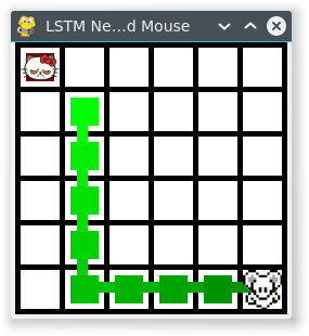
Here is an example game: (The GUI was done in pygame btw)

Cat & Mouse start randomly. Mouse is taught to run away from the stationary cat.

And here’s an example mistake that it made even after 2 million training games:

Example mistake, after 2 million training games. The mouse takes a step towards the cat.

I played about with different training rate values (alpha in the code) but the learning rate didn’t seem dependent upon it.

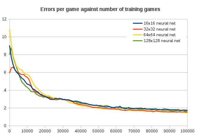
I tested increasing the hidden net from 16 to 32, and that made a pretty big difference. To reach an accuracy of 1.2 mistakes per game took:

16×16 hidden layer took 8m40s and 716342 games
32×32 hidden layer took 3m29s and 239721 games
64×64 hidden layer took 3m13s and 216513 games
128×128 hidden layer took 5m45s and 279732 games

Interestingly, if you compare the first 100,000 games the neural net size makes hardly no difference at all. They all get down to an error of about 2 at about the same rate. It’s also cool to see that the large 64×64 neural net takes about 30,000 training games to catch up with the small neural networks, since it has a much larger matrix to tame. Yet the 128×128 is much quicker to train. I don’t know why.

I also wrote a small program to display the synapses_0 matrix, which converts the input to the hidden matrix size, and plotted its against time. I also attempt to show how it is mapping the four inputs to the output by showing our four colours would be transformed by the matrix. While it is pretty to watch, it’s hard to see anything useful from it.

The synapses_0 matrix values, plotted in grayscale, and how it combines with the inputs. Each frame is 10,000 training games.

The initial and final state:

Initial random state

Final trained state, 800000 games

Graphics

For the sake of completeness, this is the graphics.py

import pygame

MAP_WIDTH = 10
MAP_HEIGHT = 10

# This sets the margin between each cell
MARGIN = 5
WINDOW_SIZE = [255, 255]

def lightened(color, amount):
  h, s, l, a = color.hsla
  if l+amount &amp;gt; 100: l = 100
  elif l+amount &amp;lt; 0: l = 0
  else: l += amount
  color.hsla = (h, s, l, a)
  return color

def init(map_width, map_height):
    global WINDOW_SIZE, MAP_WIDTH, MAP_HEIGHT, screen, clock, cat_image, mouse_image, grid_width, grid_height
    MAP_WIDTH = map_width
    MAP_HEIGHT = map_height
    grid_width = (WINDOW_SIZE[0] - MARGIN) / MAP_WIDTH - MARGIN
    grid_height = (WINDOW_SIZE[1] - MARGIN) / MAP_HEIGHT - MARGIN

    # Round the window size, so that we don't have fractions
    WINDOW_SIZE = ((grid_width + MARGIN) * MAP_WIDTH + MARGIN, (grid_height + MARGIN) * MAP_HEIGHT + MARGIN)

    # Initialize pygame
    pygame.init()
    # Set the HEIGHT and WIDTH of the screen
    screen = pygame.display.set_mode(WINDOW_SIZE)
    # Set title of screen
    pygame.display.set_caption(&amp;quot;LSTM Neural Net Cat and Mouse&amp;quot;)

    # Used to manage how fast the screen updates
    clock = pygame.time.Clock()
    cat_image = pygame.image.load(&amp;quot;cat.png&amp;quot;)
    mouse_image = pygame.image.load(&amp;quot;mouse.png&amp;quot;)

    mouse_image = pygame.transform.smoothscale(mouse_image, (grid_width, grid_height))
    cat_image = pygame.transform.smoothscale(cat_image, (grid_width, grid_height))

def updateGraphics(cat_x, cat_y, mouse_x, mouse_y):
    for event in pygame.event.get():  # User did something
        if event.type == pygame.QUIT:  # If user clicked close
            done = True  # Flag that we are done so we exit this loop
            pygame.quit()
            return False

    # Set the screen background
    screen.fill(pygame.Color(&amp;quot;black&amp;quot;))

    # Draw the grid
    for row in range(MAP_HEIGHT):
        for column in range(MAP_WIDTH):
            pygame.draw.rect(screen,
                             pygame.Color(&amp;quot;white&amp;quot;),
                             [(MARGIN + grid_width) * column + MARGIN,
                              (MARGIN + grid_height) * row + MARGIN,
                              grid_width,
                              grid_height])
    for i in range(len(mouse_x)):
        color = pygame.Color(&amp;quot;green&amp;quot;)
        color = lightened(color, -30*i/len(mouse_x))
        pygame.draw.rect(screen,
                             color,
                             [(MARGIN + grid_width) * mouse_x[i] + MARGIN*2,
                              (MARGIN + grid_height) * (MAP_HEIGHT - mouse_y[i] - 1) + MARGIN*2,
                              grid_width - MARGIN*2,
                              grid_height - MARGIN*2])
        if i != len(mouse_x) - 1:
            pygame.draw.lines(screen,
                             color,
                             False,
                             [((MARGIN + grid_width) * mouse_x[i] + (MARGIN + grid_width)/2,
                              (MARGIN + grid_height) * (MAP_HEIGHT - mouse_y[i] - 1) + (MARGIN + grid_height)/2),
                              ((MARGIN + grid_width) * mouse_x[i+1] + (MARGIN + grid_width)/2,
                              (MARGIN + grid_height) * (MAP_HEIGHT - mouse_y[i+1] - 1) + (MARGIN + grid_height)/2)],
                             10)
    for i in range(len(cat_x)):
        color = pygame.Color(&amp;quot;red&amp;quot;)
        color = lightened(color, -30*i/len(cat_x))
        pygame.draw.rect(screen,
                             color,
                             [(MARGIN + grid_width) * cat_x[i] + MARGIN*2,
                              (MARGIN + grid_height) * (MAP_HEIGHT - cat_y[i] - 1) + MARGIN*2,
                              grid_width - MARGIN*2,
                              grid_height - MARGIN*2])
        if i != len(cat_x) - 1:
            pygame.draw.lines(screen,
                             color,
                             False,
                             [((MARGIN + grid_width) * cat_x[i] + (MARGIN + grid_width)/2,
                              (MARGIN + grid_height) * (MAP_HEIGHT - cat_y[i] - 1) + (MARGIN + grid_height)/2),
                              ((MARGIN + grid_width) * cat_x[i+1] + (MARGIN + grid_width)/2,
                              (MARGIN + grid_height) * (MAP_HEIGHT - cat_y[i+1] - 1) + (MARGIN + grid_height)/2)],
                             10)
    screen.blit(mouse_image, ((MARGIN + grid_width) * mouse_x[-1] + MARGIN,
                              (MARGIN + grid_height) * (MAP_HEIGHT - mouse_y[i-1] - 1) + MARGIN))
    screen.blit(cat_image, ((MARGIN + grid_width) * cat_x[-1] + MARGIN,
                              (MARGIN + grid_height) * (MAP_HEIGHT - cat_y[i-1] - 1) + MARGIN))

    # Go ahead and update the screen with what we've drawn.
    pygame.display.flip()

    # Limit to 60 frames per second
    clock.tick(60)
    return True

What could micro-propulsion do?

November 1, 2015December 19, 2016 / John Tapsell / Leave a comment

I have been following the NASA developments on the EM Drive with great interest, and so I was very interested to see that Paul March (a NASA Eagleworks engineer) today stated that he is measuring a force of over 100µN for 80W of electrical power.

I was curious to put this into context. A quick google reveals that you can purchase solar panels for spacecraft that produce 300W/kg.

Let’s say that you can scale up the solar panels such that the mass of the engine is negligible compared to the solar panel mass. (A big assumption)

Taking his Paul March’s figure of 100µN/80W at face value, 300W per kg solar panels would produce a force per kg of = 0.0004 Newtons/kg, so an acceleration of:

$a = F/m = 0.0004 m / s^2$

This sounds extremely small, but we can accelerate constantly over long periods of time.

After 1 year of this acceleration, we would have a delta-velocity, dV, of:

$dV = at = 12 km/s$ (43,000 km/hour)

A delta-V of 12km/s isn’t shabby at all. Here’s a delta-V map of our solar system:

DeltaV map of our solar system

So from Low Earth orbit, a dV of 12km/s gets us to the moon in very low orbit, and coming back again! $(2.44+0.68+0.14+0.68+1.73 = 5.67)$

(of course you can’t actually land and take off since the force is less than that of gravity at the surface, but you could do a very low fly-by).

So we could have a shuttle going to the moon and back every year. Not sure if that’s useful, but I’m sure someone could think of a use!

What else could we do with it?

From that delta-V map, we could get to a low orbit around Venus in about 6 months $(2.44+0.68+0.09 + 0.28+0.36+2.94 = 6.79 km/s)$ .

We could get to pretty much any planet in up to a year. (e.g. low orbit Neptune is $2.44+0.68+0.09+0.39+2.7+0.99+0.69+0.27+0.35+6.75 = 15.35 km/s$ )

Imagine what we could do with a spacecraft capable of visiting the furthest planets and returning in just over a couple years.

And that’s all without any sort of gravitational slingshots!

Effect of moving away from the Sun

A reader pointed out that the solar energy collected would of course decrease as you moved away from the Sun.

We can do a quick calculation – consider a round trip to Mars and back.

Distance from Sun to Mars: 1.38 au

$(1/1.38)^2 = 52%$

So the power generated by the solar panels would be reduced by 50%. That means, roughly, on average you’d get 75% of the acceleration that I mentioned, and so would increase the round trip from lower earth orbit to lower Mars orbit from 0.95 years to 1.3 years.

(I’ve obviously linearised where I shouldn’t have, the effect being an underestimation of the time, but you can get a crude back-of-the-envelope feeling for this.)

Solar Panels or Nuclear Power?

Nasa’s “Safe Affordable Fission Engine” can generate 100kW with 500Kg mass. So 200W/kg. Less than the 300W/kg that the solar panels can produce near earth, and on par with the average for a trip to Mars. For a trip much further than the Mars then it starts to make sense.

Batteries?

Batteries store around 250Wh/kg. So 1kg can generate 250 watts for one hour… which is what a solar panel can do continuously.

Theoretical maximums

If it could be scaled to produce 1g acceleration, a human could explore this galaxy and even a neighbouring galaxy within their lifetime: http://math.ucr.edu/home/baez/physics/Relativity/SR/Rocket/rocket.html

The problem however is that at high velocities, space dust becomes more and more dangerous. At even high velocities, the very bumps in the spacetime from gravity waves becomes dangerous.

USB i2c convertor chip. A lesson in USB Latency.

October 19, 2015December 19, 2016 / John Tapsell / 1 Comment

I was interested in transmitting data from an i2c sensor to an ARM board running FreeRTOS along a long wire, and decided to use a i2c to i2c converter. Specifically a chip called MCP2221.

A single sensor reading from the i2c sensor is 2 bytes. I wanted to read 128 samples per second, so I need 256 bytes per second of data.

I figured we’d be able to do easily, what with i2c at 400khz and USB at 12 M/s. There is considerable overhead – each sensor reading needs four USB packets:

Send USB packet from arm board to usb chip telling it to read from i2c sensor
Receive ACK from USB chip
Send USB packet from arm board to usb chip telling it to send us the data that it just read
Receive the data read

Each USB packet is 64 bytes, so we have an overhead of 256 bytes for every 2 bytes of data that we want to read. This means we need a throughput of (256 bytes per sample) * (128 samples per second) = 32kb/sec.

Trying to get 32kb/s out of a 1.5MB/s USB link should be easy, I naively thought.

I wrote a driver for the chip for FreeRTOS, and tested it out.

I got a miserable 40 samples per second. Far out from the target of 128 samples per second.

So what was going wrong? Obviously I suspected a mistake with my driver. So first step is to try to reproduce on linux. I downloaded the MCP2221 Linux driver, and tested the speed of it, like so:

#!/usr/bin/env python
import smbus
import time
import sys

CONTINUOUS_MODE = True
I2C_ADDRESS = 0x48

if (len(sys.argv) == 1):
print("Please specify the bus, like:\n sudo i2c_sensor_read.py $(sudo i2cdetect -l | sed -ne 's/^i2c-\([0-9]\+\).*i2c-mcp2221.*$/\1/p')");
exit(1);

bus = smbus.SMBus(int(sys.argv[1]))

def getContinuousValue():
values = bus.read_i2c_block_data(I2C_ADDRESS, 0x0);
value = (values[0] << 8) + values[1]
return value;

last_epoch_time = 0

write_bytes([0x01, 0x4, 0x83]);
while True:
epoch_time = int(time.time()*1000);
epoch_diff = epoch_time - last_epoch_time;
last_epoch_time = epoch_time;
hz = 0;
if (epoch_diff!=0):
hz = int(1000/epoch_diff);
print str(getContinuousValue()) + " (took " + str(int(epoch_diff)) + " ms - " + str(hz) + " per second)";

This produced a miserable 62.5 samples per second. i.e. 16ms. I even tested on windows and got the same result.

So what was going on?

I tested with a oscilloscope. It was taking 1ms to send a USB packet to receive the reply, compared to the 8ms for a roundtrip that we see in the driver.

This 8ms for a roundtrip is 4ms average for sending and receiving a packet. The code in the driver (after I modified it) looks like:

static int mcp2221_ll_cmd(struct i2c_mcp2221 *dev)
{
       int rv;

       /* tell everybody to leave the URB alone */
       dev-&gt;ongoing_usb_ll_op = 1;

       /* submit the interrupt out ep packet */
       if (usb_submit_urb(dev-&gt;interrupt_out_urb, GFP_KERNEL)) {
               dev_err(&dev-&gt;interface-&gt;dev,
                               "mcp2221(ll): usb_submit_urb intr out failed\n");
               dev-&gt;ongoing_usb_ll_op = 0;
               return -EIO;
       }

       /* wait for its completion */
       rv = wait_event_interruptible(dev-&gt;usb_urb_completion_wait,
                       (!dev-&gt;ongoing_usb_ll_op));
       if (rv interface-&gt;dev, "mcp2221(ll): wait interrupted\n");
               goto ll_exit_clear_flag;
       }

       /* tell everybody to leave the URB alone */
       dev-&gt;ongoing_usb_ll_op = 1;

       /* submit the interrupt in ep packet */
       if (usb_submit_urb(dev-&gt;interrupt_in_urb, GFP_KERNEL)) {
               dev_err(&dev-&gt;interface-&gt;dev, "mcp2221(ll):
usb_submit_urb intr in failed\n");
               dev-&gt;ongoing_usb_ll_op = 0;
               return -EIO;
       }

       /* wait for its completion */
       rv = wait_event_interruptible(dev-&gt;usb_urb_completion_wait,
                       (!dev-&gt;ongoing_usb_ll_op));
       if (rv interface-&gt;dev, "mcp2221(ll): wait interrupted\n");
               goto ll_exit_clear_flag;
       }

ll_exit_clear_flag:
       dev-&gt;ongoing_usb_ll_op = 0;
       return rv;
}

I spoke to the Alan Stern and Greg KH, the Linux kernel USB maintainers, who were not surprised by this 8ms delay at all, and told me:

Why are we seeing such a large latency?
I don’t see anything wrong here, USB isn’t guaranteed to have any specific latency, what you are doing here is the worst-possible-case for a USB system (i.e. send a packet, wait for it to complete, send another one, etc.) There are lots of ways to get much better throughput if that is what you are wanting to do.

Can we make this faster?

For a horrid protocol like this, no, there isn’t any way to make it go faster, sorry. That is designed in such a way to make it the worst possible thing for a USB system, go kick the person who designed such a thing (hint, they have no idea how USB works…)

I strongly suggest going and getting a different sensor chip, don’t encourage such behaviour by actually buying their hardware.

Where is the delay coming from?

Multiple places: time to submit the request, time to reserve bandwidth for the previously unused interrupt endpoint, time to complete the transfer, all multiplied by 2.

You can get more information from usbmon (see Documentation/usb/usbmon.txt in the kernel source). But Greg is right; the protocol you described is terrible. There’s no need for a multiple ping-pong interchange like that; all you should need to do is wait for the device to send the next bit (or whatever) of data as soon as it becomes available.

Balancing on a stick

September 19, 2015December 19, 2016 / John Tapsell / Leave a comment

Consider a pole of length $h$ , with a motor and flywheel attached to one end. The motor can spin up the flywheel. The other end is on a non-slip floor.

If the stick is at angle $\theta$ , and the total mass of motor $M_m$ plus mass of flywheel, $M_f$ is $M_m + M_f = M_t$ , the torque due to gravity, $\tau_g$ is:

$\tau_g = M_t gh \cdot \sin(\theta)$

For a solid and hollow flywheel, the moment of inertia is:

$I_s = \dfrac{M_f r^2}{2}$ and $I_h = M_f r^2$

If the motor applies torque $\tau_m$ , then the angular acceleration of the flywheel is:

$\alpha = \dfrac{d\omega(t)}{dt} = \dfrac{\tau_m}{I}$

And this will require a power at time t, $P(t)$ of:

$P(t) = \tau_m \cdot \omega(t) = \tau_m \cdot \int{\dfrac{\tau_m}{I}}dt$

If we start the flywheel from rest, and keep the torque constant:

$P(t) = \dfrac{\tau_m^2}{I}\cdot t$

(In units, we’ve got on the left: $J/s = Nm/s$ and on the right $(Nm)^2 (kg^{-1} m^{-2}) s = Nm (kg m^2 s^{-2}) (kg^{-1} m^{-2}) s = Nm/s$ , thus the units match and check our work)

So the power required to keep a given torque increases linearly with time.

Notice that $I \propto M_f$ and the torque required to counter gravity is $\tau_m \propto M_t$ , so if the mass is dominated by the flywheel then $P \propto M_t$ .

So we want to minimize the mass of the flywheel (while keeping the assumption that the flywheel mass dominates the total mass) while maximizing the moment of inertia.

That means that we want to use a hollow flywheel, since this has twice the moment of inertial for a given mass.

Combining the equation $P(t)$ with the equation for $\tau_m$ , we get

$P(t) = \dfrac{\tau_m^2}{I}\cdot t = \dfrac{(M_t gh \cdot \sin(\theta))^2}{I}\cdot t = \dfrac{M_t^2 g^2h^2 \cdot \sin^2(\theta)}{I}\cdot t$

And substituting in the equation we had for $I_h = M_f r^2$:

$P(t) = \dfrac{M_t^2 g^2h^2 \cdot \sin^2(\theta)}{M_f r^2}\cdot t$

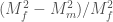
If we want to minimize the power, then we want to minimize $M_t^2/M^f = (M_m + M_f)^2/M_f$ . Differentiating gives $(M_f^2 - M_m^2)/M_f^2$ which has a zero at $M_f = M_m$ .

So the minimum power required is when $M_f = M_m$ !

Three flywheels

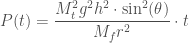
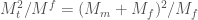
If we consider the case of having two or three flywheels on the box, perpendicular to each other to give us more control, then we can consider each flywheel individually, and consider $M_m$ to include the mass of the other flywheels. For minimum power usage, this would mean that we’d want to minimize $(M_m + 3M_f)^2/M_f$ which is minimum at $M_f = M_m/3$.

So if we have 1kg of motors, payload, etc, then we’d want the flywheels to be 1/3 kg each.

Radius of flywheel

Since $P \propto 1/r^2$ we want to maximize the radius of the flywheel.

Example

A random example EDF motor has weight 148 grams (which we’ll round up to 0.2kg) and produces 450 Watts of power. We’ll consider this on a stick of length 1 meter and with a hollow flywheel.

If we begin at an angle of 10 degrees (0.17 radians) and desire a torque sufficient to balance against gravity:

$\tau_g = (M_f + M_m) gh \cdot \sin(\theta) = (M_f + M_m) \cdot (1m * 10m/s^2) \cdot 0.17 = (M_f + M_m) \cdot (1.7m^2/s^2)$

So:

$P(t) = \dfrac{\tau_m^2}{I}\cdot t = \dfrac{(M_f + M_m)^2 \cdot (2.89 m^4/s^4)}{M_f r^2} \cdot t$

Let’s make the radius 0.1m – i.e. 10% of the length of the stick. We’ll consider the case of using a single flywheel and minimizing the power usage.

So this gives a power of $P(t) = (2M_f)^2/M_f \cdot (0.0289 m^2/s^4) \cdot t = 4 M_f \cdot (0.0289 m^2/s^4) \cdot t = M_f \cdot (0.1156 m^2/s^4) \cdot t$

Using the EDF motor mass of 0.2kg:

$P(t) = (0.023 kg m^2/s^4) \cdot t = (0.023 J/s^2) \cdot t$

The motor can provide a maximum of 450 Watts, meaning that it could maintain a 10 degree angle for 450/0.023 s = 19565 seconds = 5.4 hours.

	Bilal on Update: Release! ChatGPT clone…
	moon on Nokia 6110 Part 3 –…
	Lee V on Adobe After Effects
	John Tapsell on Nokia 6110 Part 3 –…
	Quackleb on Nokia 6110 Part 3 –…